Derivation: Maximum Likelihood for Boltzmann Machines

In this post I will review the gradient descent algorithm that is commonly used to train the general class of models known as Boltzmann machines. Though the primary goal of the post is to supplement another post on restricted Boltzmann machines, I hope that those readers who are curious about how Boltzmann machines are trained, but have found it difficult to track down a complete or straight-forward derivation of the maximum likelihood learning algorithm for these models (as I have), will also find the post informative.

First, a little background: Boltzmann machines are stochastic neural networks that can be thought of as the probabilistic extension of the Hopfield network. The goal of the Boltzmann machine is to model a set of observed data in terms of a set of visible random variables  and a set of latent/unobserved random variables . Due to the relationship between Boltzmann machines and neural networks, the random variables are often are often referred to as “units.” The role of the visible units is to approximate the true distribution of the data, while the role of the latent variables it to extend the expressiveness of the model by capturing underlying features in the observed data. The latent variables are often referred to as hidden units, as they do not result directly from the observed data and are generally marginalized over to obtain the likelihood of the observed data,  i.e.

,

 

where is the joint probability distribution over the visible and hidden units based on the current model parameters . The general Boltzmann machine defines through a set of weighted,  symmetric connections between all visible and hidden units (but no connections from any unit to itself). The graphical model for the general Boltzmann machine is shown in Figure 1.

Figure 1: Graphical Model of the Boltzmann machine (biases not depicted).

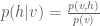
Given the current state of the visible and hidden units, the overall configuration of the model network is described by a connectivity function , parameterized by :

The parameter matrix defines the connection strength between the visible and hidden units. The parameters and define the connection strength amongst hidden units and visible units, respectively. The model also includes a set of  biases and that capture offsets for each of the hidden and visible units.

The Boltzmann machine has been used for years in field of statistical mechanics to model physical systems based on the principle of energy minimization. In the statistical mechanics, the connectivity function is often referred to the “energy function,” a term that is has also been standardized in the statistical learning literature. Note that the energy function returns a single scalar value for any configuration of the network parameters and random variable states.

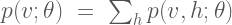
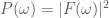
Given the energy function, the Boltzmann machine models the joint probability of the visible and hidden unit states as a Boltzmann distribution:

The partition function is a normalizing constant that is calculated by summing over all possible states of the network . Here we assume that all random variables take on discrete values, but the analogous derivation holds for continuous or mixed variable types by replacing the sums with integrals accordingly.

The common way to train the Boltzmann machine is to determine the parameters that maximize the likelihood of the observed data. To determine the parameters, we perform gradient descent on the log of the likelihood function (In order to simplify the notation in the remainder of the derivation, we do not include the explicit dependency on the parameters . To further simplify things, let’s also assume that we calculate the gradient of the likelihood based on a single observation.):

The gradient calculation is as follows:

Here we can simplify the expression somewhat by noting that , that , and also that is a constant:

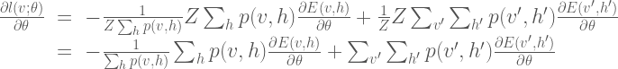
If we also note that , and use the definition of conditional probability , we can further simplify the expression for the gradient:

Here is the expected value under the distribution . Thus the gradient of the likelihood function is composed of two parts. The first part is expected gradient of the energy function with respect to the conditional distribution . The second part is expected gradient of the energy function with respect to the joint distribution over all variable states. However, calculating these expectations is generally infeasible for any realistically-sized model, as it involves summing over a huge number of possible states/configurations. The general approach for solving this problem is to use Markov Chain Monte Carlo (MCMC) to approximate these sums:

Here is the sample average of samples drawn according to the process . The first term is calculated by taking the average value of the energy function gradient when the visible and hidden units are being driven by observed data samples. In practice, this first term is generally straightforward to calculate. Calculating the second term is generally more complicated and involves running a set of Markov chains until they reach the current model’s equilibrium distribution (i.e. via Gibbs sampling, Metropolis-Hastings, or the like), then taking the average energy function gradient based on those samples. See this post on MCMC methods for details. It turns out that there is a subclass of Boltzmann machines that, due to a restricted connectivity/energy function (specifically, the parameters ), allow for efficient MCMC by way of blocked Gibbs sampling. These models, known as restricted Boltzman machines have become an important component for unsupervised pretraining in the field of deep learning and will be the focus of a related post.

A Gentle Introduction to Artificial Neural Networks

The material in this post has been migrated to a post by the same name on my github pages website.

Derivation: Derivatives for Common Neural Network Activation Functions

The material in this post has been migraged with python implementations to my github pages website.

Derivation: Error Backpropagation & Gradient Descent for Neural Networks

The material in this post has been migraged with python implementations to my github pages website.

Model Selection: Underfitting, Overfitting, and the Bias-Variance Tradeoff

The material in this post has been migrated with python implementations to my github pages website.

fMRI In Neuroscience: Efficiency of Event-related Experiment Designs

Event-related fMRI experiments are used to detect selectivity in the brain to stimuli presented over short durations. An event is generally modeled as an impulse function that occurs at the onset of the stimulus in question. Event-related designs are flexible in that many different classes of stimuli can be intermixed. These designs can minimize confounding behavioral effects due to subject adaptation or expectation. Furthermore, stimulus onsets can be modeled at frequencies that are shorter than the repetition time (TR) of the scanner. However, given such flexibility in design and modeling, how does one determine the schedule for presenting a series of stimuli? Do we space out stimulus onsets periodically across a scan period? Or do we randomize stimulus onsets? Furthermore what is the logic for or against either approach? Which approach is more efficient for gaining incite into the selectivity in the brain?

Simulating Two fMRI Experiments: Periodic and Random Stimulus Onsets

To get a better understanding of the problem of choosing efficient experiment design, let’s simulate two simple fMRI experiments. In the first experiment, a stimulus is presented periodically 20 times, once every 4 seconds, for a run of 80 seconds in duration. We then simulate a noiseless BOLD signal evoked in a voxel with a known HRF. In the second experiment, we simulate the noiseless BOLD signal evoked by 20 stimulus onsets that occur at random times over the course of the 80 second run duration.  The code for simulating the signals and displaying output are shown below:

rand('seed',12345);
randn('seed',12345);
TR = 1 % REPETITION TIME
t = 1:TR:20; % MEASUREMENTS
h = gampdf(t,6) + -.5*gampdf(t,10); % ACTUAL HRF
h = h/max(h); % SCALE TO MAX OF 1

% SOME CONSTANTS...
trPerStim = 4; % # TR PER STIMULUS FOR PERIODIC EXERIMENT
nRepeat = 20; % # OF TOTAL STIMULI SHOWN
nTRs = trPerStim*nRepeat
stimulusTrain0 = zeros(1,nTRs);

beta = 3; % SELECTIVITY/HRF GAIN

% SET UP TWO DIFFERENT STIMULUS PARADIGM...
% A. PERIODIC, NON-RANDOM STIMULUS ONSET TIMES
D_periodic = stimulusTrain0;
D_periodic(1:trPerStim:trPerStim*nRepeat) = 1;

% UNDERLYING MODEL FOR (A)
X_periodic = conv2(D_periodic,h);
X_periodic = X_periodic(1:nTRs);
y_periodic = X_periodic*beta;

% B. RANDOM, UNIFORMLY-DISTRIBUTED STIMULUS ONSET TIMES
D_random = stimulusTrain0;
randIdx = randperm(numel(stimulusTrain0)-5);
D_random(randIdx(1:nRepeat)) = 1;

% UNDERLYING MODEL FOR (B)
X_random = conv2(D_random,h);
X_random = X_random(1:nTRs);
y_random = X_random*beta;

% DISPLAY STIMULUS ONSETS AND EVOKED RESPONSES
% FOR EACH EXPERIMENT
figure
subplot(121)
stem(D_periodic,'k');
hold on;
plot(y_periodic,'r','linewidth',2);
xlabel('Time (TR)');
title(sprintf('Responses Evoked by\nPeriodic Stimulus Onset\nVariance=%1.2f',var(y_periodic)))

subplot(122)
stem(D_random,'k');
hold on;
plot(y_random,'r','linewidth',2);
xlabel('Time (TR)');
title(sprintf('Responses Evoked by\nRandom Stimulus Onset\nVariance=%1.2f',var(y_random)))

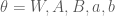
BOLD signals evoked by periodic (left) and random (right) stimulus onsets.

The black stick functions in the simulation output indicate the stimulus onsets and each red function is the simulated noiseless BOLD signal to those stimuli. The first thing to notice is the dramatically different variances of the BOLD signals evoked for the two stimulus presentation schedules. For the periodic stimuli, the BOLD signal quickly saturates, then oscillates around an effective baseline activation. The estimated variance of the periodic-based signal is 0.18. In contrast, the signal evoked by the random stimulus presentation schedule varies wildly, reaching a maximum amplitude that is roughly 2.5 times as large the maximum amplitude of the signal evoked by periodic stimuli. The estimated variance of the signal evoked by the random stimuli is 7.4, roughly 40 times the variance of the signal evoked by the periodic stimulus.

So which stimulus schedule allows us to better estimate the HRF and, more importantly, the amplitude of the HRF, as it is the amplitude that is the common proxy for voxel selectivity/activation? Below we repeat the above experiment 50 times. However, instead of simulating noiseless BOLD responses, we introduce 50 distinct, uncorrelated noise conditions, and from the simulated noisy responses, we estimate the HRF using an FIR basis set for each  repeated trial. We then compare the estimated HRFs across the 50 trials for the periodic and random stimulus presentation schedules. Note that for each trial, the noise is exactly the same for the two stimulus presentation schedules. Further, we simulate a selectivity/tuning gain of 3 times the maximum HRF amplitude and assume that the HRF to be estimated is 16 TRs/seconds in length. The simulation and output are below:

%% SIMULATE MULTIPLE TRIALS OF EACH EXPERIMENT
%% AND ESTIMATE THE HRF FOR EACH
%% (ASSUME THE VARIABLES DEFINED ABOVE ARE IN WORKSPACE)

% CREATE AN FIR DESIGN MATRIX
% FOR EACH EXPERIMENT
hrfLen = 16;  % WE ASSUME TO-BE-ESTIMATED HRF IS 16 TRS LONG

% CREATE FIR DESIGN MATRIX FOR THE PERIODIC STIMULI
X_FIR_periodic = zeros(nTRs,hrfLen);
onsets = find(D_periodic);
idxCols = 1:hrfLen;
for jO = 1:numel(onsets)
	idxRows = onsets(jO):onsets(jO)+hrfLen-1;
	for kR = 1:numel(idxRows);
		X_FIR_periodic(idxRows(kR),idxCols(kR)) = 1;
	end
end
X_FIR_periodic = X_FIR_periodic(1:nTRs,:);

% CREATE FIR DESIGN MATRIX FOR THE RANDOM STIMULI
X_FIR_random = zeros(nTRs,hrfLen);
onsets = find(D_random);
idxCols = 1:hrfLen;
for jO = 1:numel(onsets)
	idxRows = onsets(jO):onsets(jO)+hrfLen-1;
	for kR = 1:numel(idxRows);
		X_FIR_random(idxRows(kR),idxCols(kR)) = 1;
	end
end
X_FIR_random = X_FIR_random(1:nTRs,:);

% SIMULATE AND ESTIMATE HRF WEIGHTS VIA OLS
nTrials = 50;

% CREATE NOISE TO ADD TO SIGNALS
% NOTE: SAME NOISE CONDITIONS FOR BOTH EXPERIMENTS
noiseSTD = beta*2;
noise = bsxfun(@times,randn(nTrials,numel(X_periodic)),noiseSTD);

%% ESTIMATE HRF FROM PERIODIC STIMULUS TRIALS
beta_periodic = zeros(nTrials,hrfLen);
for iT = 1:nTrials
	y = y_periodic + noise(iT,:);
	beta_periodic(iT,:) = X_FIR_periodic\y';
end

% CALCULATE MEAN AND STANDARD ERROR OF HRF ESTIMATES
beta_periodic_mean = mean(beta_periodic);
beta_periodic_se = std(beta_periodic)/sqrt(nTrials);

%% ESTIMATE HRF FROM RANDOM STIMULUS TRIALS
beta_random = zeros(nTrials,hrfLen);
for iT = 1:nTrials
	y = y_random + noise(iT,:);
	beta_random(iT,:) = X_FIR_random\y';
end

% CALCULATE MEAN AND STANDARD ERROR OF HRF ESTIMATES
beta_random_mean = mean(beta_random);
beta_random_se = std(beta_random)/sqrt(nTrials);

% DISPLAY HRF ESTIMATES
figure
% ...FOR THE PERIODIC STIMULI
subplot(121);
hold on;
h0 = plot(h*beta,'k')
h1 = plot(beta_periodic_mean,'linewidth',2);
h2 = plot(beta_periodic_mean+beta_periodic_se,'r','linewidth',2);
plot(beta_periodic_mean-beta_periodic_se,'r','linewidth',2);
xlabel('Time (TR)')
legend([h0, h1,h2],'Actual HRF','Average \beta_{periodic}','Standard Error')
title('Periodic HRF Estimate')

% ...FOR THE RANDOMLY-PRESENTED STIMULI
subplot(122);
hold on;
h0 = plot(h*beta,'k');
h1 = plot(beta_random_mean,'linewidth',2);
h2 = plot(beta_random_mean+beta_random_se,'r','linewidth',2);
plot(beta_random_mean-beta_random_se,'r','linewidth',2);
xlabel('Time (TR)')
legend([h0,h1,h2],'Actual HRF','Average \beta_{random}','Standard Error')
title('Random HRF Estimate')

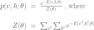
Estimated HRFs from 50 trials of periodic (left) and random (right) stimulus schedules

In the simulation outputs, the average HRF for the random stimulus presentation (right) closely follows the actual HRF tuning. Also, there is little variability of the HRF estimates, as is indicated by the small standard error estimates for each time points. As well, the selectivity/gain term is accurately recovered, giving a mean HRF with nearly the same amplitude as the underlying model. In contrast, the HRF estimated from the periodic-based experiment is much more variable, as indicated by the large standard error estimates. Such variability in the estimates of the HRF reduce our confidence in the estimate for any single trial. Additionally, the scale of the mean HRF estimate is off by nearly 30% of the actual value.

From these results, it is obvious that the random stimulus presentation rate gives rise to more accurate, and less variable estimates of the HRF function. What may not be so obvious is why this is the case, as there were the same number of stimuli and  the same number of signal measurements in each experiment. To get a better understanding of why this is occurring, let’s refer back to the variances of the evoked noiseless signals. These are the signals that are underlying the noisy signals used to estimate the HRF. When noise is added it impedes the detection of the underlying trends that are useful for estimating the HRF.  Thus it is important that the variance of the underlying signal is large compared to the noise so that the signal can be detected.

For the periodic stimulus presentation schedule, we saw that the variation in the BOLD signal was much smaller than the variation in the BOLD signals evoked during the randomly-presented stimuli. Thus the signal evoked by random stimulus schedule provide a better characterization of the underlying signal in the presence of the same amount of noise, and thus provide more information to estimate the HRF. With this in mind we can think of maximizing the efficiency of the an experiment design as maximizing the variance of the BOLD signals evoked by the experiment.

An Alternative Perspective: The Frequency Power Spectrum

Another helpful interpretation is based on a signal processing perspective. If we assume that neural activity is directly correspondent with the onset of a stimulus event, then we can interpret the train of stimulus onsets as a direct signal of the evoked neural activity. Furthermore, we can interpret the HRF as a low-pass-filter that acts to “smooth” the available neural signal in time. Each of these signals–the neural/stimulus signal and the HRF filtering signal–has with it an associated power spectrum. The power spectrum for a signal captures the amount of power per unit time that the signal has as a particular frequency . The power spectrum for a discrete signal can be calculated from the discrete Fourier transform (DFT) of the signal as follows

Below, we use Matlab’s function to calculate the DFT and the associated power spectrum for each of the stimulus/neural signals, as well as the HRF.

%% POWER SPECTRUM ANALYSES
%% (ASSUME THE VARIABLES DEFINED ABOVE ARE IN WORKSPACE)

% MAKE SURE WE PAD SUFFICIENTLY
% FOR CIRCULAR CONVOLUTION
N = 2^nextpow2(nTRs + numel(h)-1);
nUnique = ceil(1+N/2); % TAKE ONLY POSITIVE SPECTRA

% CALCULATE POWER SPECTRUM FOR PERIODIC STIMULI EXPERIMENT
ft_D_periodic = fft(D_periodic,N)/N; % DFT
P_D_periodic = abs(ft_D_periodic).^2; % POWER
P_D_periodic = 2*P_D_periodic(2:nUnique-1); % REMOVE ZEROTH & NYQUIST

% CALCULATE POWER SPECTRUM FOR RANDOM STIMULI EXPERIMENT
ft_D_random = fft(D_random,N)/N; % DFT
P_D_random = abs(ft_D_random).^2; % POWER
P_D_random = 2*P_D_random(2:nUnique-1); % REMOVE ZEROTH & NYQUIST

% CALCULATE POWER SPECTRUM OF HRF
ft_h = fft(h,N)/N; % DFT
P_h = abs(ft_h).^2; % POWER
P_h = 2*P_h(2:nUnique-1); % REMOVE ZEROTH & NYQUIST

% CREATE A FREQUENCY SPACE FOR PLOTTING
F = 1/N*[1:N/2-1];

% DISPLAY STIMULI POWER SPECTRA
figure
subplot(131)
hhd = plot(F,P_D_periodic,'b','linewidth',2);
axis square; hold on;
hhr = plot(F,P_D_random,'g','linewidth',2);
xlim([0 .3]); xlabel('Frequency (Hz)');
set(gca,'Ytick',[]); ylabel('Magnitude');
legend([hhd,hhr],'Periodic','Random')
title('Stimulus Power, P_{stim}')

% DISPLAY HRF POWER SPECTRUM
subplot(132)
plot(F,P_h,'r','linewidth',2);
axis square
xlim([0 .3]); xlabel('Frequency (Hz)');
set(gca,'Ytick',[]); ylabel('Magnitude');
title('HRF Power, P_{HRF}')

% DISPLAY EVOKED SIGNAL POWER SPECTRA
subplot(133)
hhd = plot(F,P_D_periodic.*P_h,'b','linewidth',2);
hold on;
hhr = plot(F,P_D_random.*P_h,'g','linewidth',2);
axis square
xlim([0 .3]); xlabel('Frequency (Hz)');
set(gca,'Ytick',[]); ylabel('Magnitude');
legend([hhd,hhr],'Periodic','Random')
title('Signal Power, P_{stim}.*P_{HRF}')

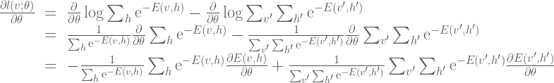
Power spectrum of neural/stimulus (left), HRF (center), and evoked BOLD (right) signals

On the left of the output we see the power spectra for the stimulus signals. The blue line corresponds to the spectrum for the periodic stimuli, and the green line the spectrum for the randomly-presented stimuli. The large peak in the blue spectrum corresponds to the majority of the stimulus power at 0.25 Hz for the periodic stimuli, as this the fundamental frequency of the periodic stimulus presentation (i.e. every 4 seconds). However, there is little power at any other stimulus frequencies. In contrast the green spectrum indicates that the random stimulus presentation has power at multiple frequencies.

If we interpret the HRF as a filter, then we can think of the HRF power spectrum as modulating the power spectrum of the neural signals to produce the power of the evoked BOLD signals. The power spectrum for the HRF is plotted in red in the center plot. Notice how a majority of the power for the HRF is at frequencies less than 0.1 Hz, and there is very little power at frequencies above 0.2 Hz. If the neural signal power is modulated by the HRF signal power, we see that there is little resultant power in the BOLD signals evoked by periodic stimulus presentation (blue spectrum in the right plot). In contrast, because the power for the neural signals evoked by random stimuli are spread across the frequency domain, there are a number of frequencies that overlap with those frequencies for which the HRF also has power. Thus after modulating neural/stimulus power with the HRF power, the spectrum of the BOLD signals evoked by the randomly-presented stimuli have much more power across the relevant frequency spectrum than those evoked by the periodic stimuli. This is indicated by the larger area under the green curve in the right plot.

Using the signal processing perspective allows us to directly gain perspective on the limitations of a particular experiment design which are rooted in the frequency spectrum of the HRF. Therefore, another way we can think of maximizing the efficiency of an experimental design is maximizing the amount of power in the resulting evoked BOLD responses.

Yet Another Perspective Based in Statistics: Efficiency Metric

Taking a statistics-based approach leads to a formal definition of efficiency, and further, a nice metric for testing the efficiency of an experimental design. Recall that when determining the shape of the HRF, a common approach is to use the GLM model

Here is the evoked BOLD signal and is a design matrix that links a set of linear model parameters to those responses. The variable is a noise term that is unexplained by the model. Using an FIR basis formulation of the model, the weights in represent the HRF to a stimulus condition.

Because fMRI data are a continuous time series, the underlying noise is generally correlated in time. We can model this noise as a Gaussian process with zero mean and a constant multivariate covariance . Note that this is analogous to the Generalized Least Squares (GLS) formulation of the GLM. In general, the values that comprise are unknown and have to be estimated from the fMRI data themselves.

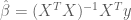
For a known or estimated noise covariance, the Maximum Likelihood Estimator (MLE) for the model parameters (derivation not shown) is:

Because the ML estimator of the HRF is a linear combination of the design matrix and a set of corresponding responses, which are both random variables ( can represent any possible experiment design, and is by definition random), the estimator is itself a random variable. It thus follows that the estimate for the HRF also has a variance. (We demonstrated how is a random variable in the 50 simulations above, where for each simulation X was held fixed, but due to the added noise was a random variable. For each noise condition, the estimate for took on different values.) We saw above how an HRF estimator with a large variance is undesirable, as it reduces our confidence in the estimates of the HRF shape and scale. Therefore we would like to determine an estimator that has a minimum overall variance.

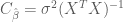
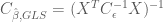
A formal metric for efficiency of a least-squares estimator is directly related to the variance of the estimator. The efficiency is defined to be the inverse of the sum of the estimator variances. An estimator that has a large sum of variances will have a low efficiency, and vice versa. But how do we obtain the values of the variances for the estimator? The variances can be recovered from the diagonal elements of the estimator covariance matrix , giving the following definition for the efficiency,

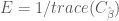
In earlier post we found that the covariance matrix for the GLS estimator (i.e. the formulation above) with a given noise covariance is:

.

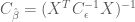
Thus the efficiency for the HRF estimator is

Here we see that the efficiency depends only on the known noise covariance (or an estimate of it), and the design matrix used in the model, but not the shape of the HRF. In general the noise covariance is out of the experimenter’s control (but see the take-homes below ), and must be dealt with post hoc. However, because the design matrix is directly related to the experimental design, the above expression gives a direct way to test the efficiency of experimental designs before they are ever used!

In the simulations above, the noise processes are drawn from an independent multivariate Gaussian distribution, therefore the noise covariance is equal to the identity (i.e. uncorrelated). We also estimated the HRF using the FIR basis set, thus our model design matrix was . This gives the estimate the efficiency for the simulation experiments:

Below we calculate the efficiency for the FIR estimates under the simulated experiments with periodic and random stimulus presentation designs.

%% ESTIMATE DESIGN EFFICIENCY
%% (ASSUME THE VARIABLES DEFINED ABOVE ARE IN WORKSPACE)

% CALCULATE EFFICIENCY OF PERIODIC EXPERIMENT
E_periodic = 1/trace(pinv(X_FIR_periodic'*X_FIR_periodic));

% CALCULATE EFFICIENCY OF RANDOM EXPERIMENT
E_random = 1/trace(pinv(X_FIR_random'*X_FIR_random));

% DISPLAY EFFICIENCY ESTIMATES
figure
bar([E_periodic,E_random]);
set(gca,'XTick',[1,2],'XTickLabel',{'E_periodic','E_random'});
title('Efficiency of Experimental Designs');
colormap hot;

Estimated efficiency for simulated periodic (left) and random (right) stimulus schedules.

Here we see that the efficiency metric does indeed indicate that the randomly-presented stimulus paradigm is far more efficient than the periodically-presented paradigm.

Wrapping Up

In this post we addressed the efficiency of an fMRI experiment design. A few take-homes from the discussion are:

1. Randomize stimulus onset times. These onset times should take into account the low-pass characteristics (i.e. the power spectrum) of the HRF.
2. Try to model selectivity to events that occur close in time. The reason for this is that noise covariances in fMRI are highly non-stationary. There are many sources of low-frequency physiological noise such as breathing, pulse, blood pressure, etc, all of which dramatically effect the noise in the fMRI timecourses. Thus any estimate of noise covariances from data recorded far apart in time will likely be erroneous.
3. Check an experimental design against other candidate designs using the Efficiency metric.

Above there is mention of the effects of low-frequency physiological noise. Until now, our simulations have assumed that all noise is independent in time, greatly simplifying the picture of estimating HRFs and corresponding selectivity. However, in a later post we’ll address how to deal with more realistic time courses that are heavily influenced by sources of physiological noise. Additionally, we’ll tackle how to go about estimating the noise covariance from more realistic fMRI time series.

Derivation: The Covariance Matrix of an OLS Estimator (and applications to GLS)

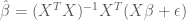
We showed in an earlier post that for the linear regression model

,

the optimal Ordinary Least Squares (OLS) estimator for model parameters is

However, because independent variables and responses can take on any value, they are both random variables. And, because is a linear combination of and , it is also a random variable, and therefore has a covariance. The definition of the covariance matrix for the OLS estimator is defined as:

where, denotes the expected value operator. In order to find an expression for , we first need an expression for  . The following derives this expression:

,

where we use the fact that

.

It follows that

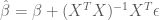
and therefore

Now following the original definition for …

where we take advantage of in order to rewrite the second term in the product of the expectation. If we take to be fixed for a given estimator of (in other words we don’t randomly resample the independent variables), then the expectation only depends on the remaining stochastic/random variable, namely . Therefore the above expression can be written as

.

where is the covariance of the noise term in the model. Because OLS assumes uncorrelated noise, the noise covariance is equal to , where is the variance along each dimension, and is an identity matrix of size equal to the number of dimensions. The expression for the estimator covariance is now:

,

which simplifies to

A further simplifying assumption made by OLS that is often made is that is drawn from a zero mean multivariate Guassian distribution of unit variances (i.e. ), resulting in a noise covariance equal to the identity. Thus

Applying the derivation results to Generalized Least Squares

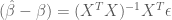
Notice that the expression for the OLS estimator covariance is equal to first inverse term in the expression for the OLS estimator. Identitying the covariance for the OLS estimator in this way gives a helpful heuristic to easily identify the covariance of related estimators that do not make the simplifying assumptions about the covariance that are made in OLS. For instance in Generalized Least Squares (GLS), it is possible for the noise terms to co-vary. The covariance is represented as a noise covariance matrix . This gives the model form

,

where .

In otherwords, under GLS, the noise terms have zero mean, and covariance .  It turns out that estimator for the GLS model parameters is

.

Notice the similarity between the GLS and OLS estimators. The only difference is that in GLS, the solution for the parameters is scaled by the inverse of the noise covariance. And, in a similar fashion to the OLS estimator, the covariance for the GLS estimator is first term in the product that defines the GLS estimator:

Basis Function Models

Often times we want to model data that emerges from some underlying function of independent variables such that for some future input we’ll be able to accurately predict the future output values. There are various methods for devising such a model, all of which make particular assumptions about the types of functions the model can emulate. In this post we’ll focus on one set of methods called Basis Function Models (BFMs).

Basis Sets and Linear Independence

The idea behind BFMs is to model the complex target function as a linear combination of a set of simpler functions, for which we have closed form expressions. This set of simpler functions is called a basis set, and work in a similar manner to bases that compose vector spaces in linear algebra. For instance, any vector in the 2D spatial coordinate system (which is a vector space in  ) can be composed of linear combinations of the and directions. This is demonstrated in the figures below:

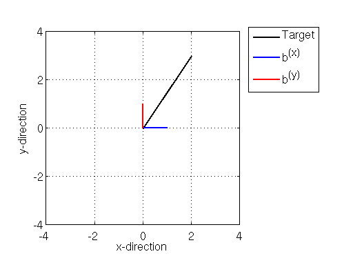
Illustration of basis vectors along the x (blue) and y(red) directions, along with a target vector (black)

Above we see a target vector in black pointing from the origin (at xy coordinates (0,0)) to the xy coordinates (2,3), and the coordinate basis vectors and , each of which point one unit along the x- (in blue) and y- (in red) directions.

We can compose the target vector as as a linear combination of the x- and y- basis vectors. Namely the target vector can be composed by adding (in the vector sense) 2 times the basis to 3 times the basis :

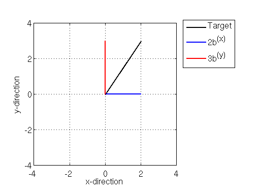
Composing the target vector as a linear combination of the basis vectors

One thing that is important to note about the bases and is that they are linearly independent. This means that no matter how hard you try, you can’t compose the basis vector as a linear combination of the other basis vector , and vice versa. In the 2D vector space, we can easily see this because the red and blue lines are perpendicular to one another (a condition called orthogonality). But we can formally determine if two (column) vectors are independent by calculating the (column) rank of a matrix that is composed by concatenating the two vectors.

The rank of a matrix is the number of linearly independent columns in the matrix. If the rank of has the same value as the number of columns in the matrix, then the columns of    forms a linearly independent set of vectors. The rank of above is 2. So is the number of columns. Therefore the basis vectors and are indeed linearly independent. We can use this same matrix rank-based test to verify if vectors of  much higher dimension than two are independent. Linear independence of the basis set is important if we want to be able to define a unique model.

%% EXAMPLE OF COMPOSING A VECTOR OF BASIS VECTORS
figure;
targetVector = [0 0; 2 3]
basisX = [0 0; 1 0];
basisY = [0 0; 0 1];
hv = plot(targetVector(:,1),targetVector(:,2),'k','Linewidth',2)
hold on;
hx = plot(basisX(:,1),basisX(:,2),'b','Linewidth',2);
hy = plot(basisY(:,1),basisY(:,2),'r','Linewidth',2);
xlim([-4 4]); ylim([-4 4]);
xlabel('x-direction'), ylabel('y-direction')
axis square
grid
legend([hv,hx,hy],{'Target','b^{(x)}','b^{(y)}'},'Location','bestoutside');

figure
hv = plot(targetVector(:,1),targetVector(:,2),'k','Linewidth',2);
hold on;
hx = plot(2*basisX(:,1),2*basisX(:,2),'b','Linewidth',2);
hy = plot(3*basisY(:,1),3*basisY(:,2),'r','Linewidth',2);
xlim([-4 4]); ylim([-4 4]);
xlabel('x-direction'), ylabel('y-direction');
axis square
grid
legend([hv,hx,hy],{'Target','2b^{(x)}','3b^{(y)}'},'Location','bestoutside')

A = [1 0;
0 1];

% TEST TO SEE IF basisX AND basisY ARE
% LINEARLY INDEPENDENT
isIndependent = rank(A) == size(A,2)

Modeling Functions with Linear Basis Sets

In a similar fashion to creating arbitrary vectors with vector bases, we can compose arbitrary functions in “function space” as a linear combination of simpler basis functions  (note that basis functions are also sometimes called kernels). One such set of basis functions is the set of polynomials:

Here each basis function is a polynomial of order . We can then compose a basis set of  functions, where the function is , then model the function as a linear combinations of these polynomial bases:

where is the weight on the -th basis function. In matrix format this model takes the form

Here, again the matrix is the concatenation of each of the polynomial bases into its columns. What we then want to do is determine all the weights such that is as close to as possible. We can do this by using Ordinary Least Squares (OLS) regression, which was discussed in earlier posts. The optimal solution for the weights under OLS is:

Let’s take a look at a concrete example, where we use a set of  polynomial basis functions to model a complex data trend.

Example: Modeling with Polynomial Basis Functions

In this example we model a set of data whose underlying function is:

In particular we’ll create a polynomial basis set of degree 10 and fit the weights using OLS. The Matlab code for this example, and the resulting graphical output are below:

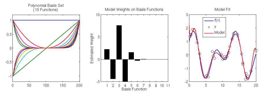
Left: Basis set of 10 (scaled) polynomial functions. Center: estimated model weights for basis set. Right: Underlying model f(x) (blue), data sampled from the model (black circles), and the linear basis model fit (red).

%% EXAMPLE: MODELING A TARGET FUNCTION
x = [0:.1:20]';
f = inline('cos(.5*x) + sin(x)','x');

% CREATE A POLYNOMIAL BASIS SET
polyBasis = [];
nPoly = 10;
px = linspace(-10,10,numel(x))';
for iP = 1:nPoly
	polyParams = zeros(1,nPoly);
	polyParams(iP) = 1;
	polyBasis = [polyBasis,polyval(polyParams,px)];
end

% SCALE THE BASIS SET TO HAVE MAX AMPLTUDE OF 1
polyBasis = fliplr(bsxfun(@rdivide,polyBasis,max(polyBasis)));

% CHECK LINEAR INDEPENDENCE
isIndependent = rank(polyBasis) == size(polyBasis,2)

% SAMPLE SOME DATA FROM THE TARGET FUNCTION
randIdx = randperm(numel(x));
xx = x(randIdx(1:30));
y = f(xx) + randn(size(xx))*.2;

% FIT THE POLYNOMIAL BASIS MODEL TO THE DATA(USING polyfit.m)
basisWeights = polyfit(xx,y,nPoly);

% MODEL OF TARGET FUNCTION
yHat = polyval(basisWeights,x);

% DISPLAY BASIS SET AND AND MODEL
subplot(131)
plot(polyBasis,'Linewidth',2)
axis square
xlim([0,numel(px)])
ylim([-1.2 1.2])
title(sprintf('Polynomial Basis Set\n(%d Functions)',nPoly))

subplot(132)
bar(fliplr(basisWeights));
axis square
xlim([0 nPoly + 1]); colormap hot
xlabel('Basis Function')
ylabel('Estimated Weight')
title('Model Weights on Basis Functions')

subplot(133);
hy = plot(x,f(x),'b','Linewidth',2); hold on
hd = scatter(xx,y,'ko');
hh = plot(x,yHat,'r','Linewidth',2);
xlim([0,max(x)])
axis square
legend([hy,hd,hh],{'f(x)','y','Model'},'Location','Best')
title('Model Fit')
hold off;

First off, let’s make sure that the polynomial basis is indeed linearly independent. As above, we’ll compute the rank of the matrix composed of the basis functions along its columns. The rank of the basis matrix has a value of 10, which is also the number of columns of the matrix (line 19 in the code above). This proves that the basis functions are linearly independent.

We fit the model using Matlab’s internal function , which performs OLS on the basis set matrix. We see that the basis set of 10 polynomial functions (including the zeroth-bias term) does a pretty good job of modeling a very complex function . We essentially get to model a highly nonlinear function using simple linear regression (i.e. OLS).

Wrapping up

Though the polynomial basis set works well in many modeling problems, it may be a poor fit for some applications. Luckily we aren’t limited to using only polynomial basis functions. Other basis sets include Gaussian basis functions, Sigmoid basis functions, and finite impulse response (FIR) basis functions, just to name a few (a future post, we’ll demonstrate how the FIR basis set can be used to model the hemodynamic response function (HRF) of an fMRI voxel measured from brain).

fMRI in Neuroscience: Estimating Voxel Selectivity & the General Linear Model (GLM)

In a typical fMRI experiment  a series of stimuli are presented to an observer and evoked brain activity–in the form of blood-oxygen-level-dependent (BOLD) signals–are measured from tiny chunks of the brain called voxels. The task of the researcher is then to infer the tuning of the voxels to features in the presented stimuli based on the evoked BOLD signals. In order to make this inference quantitatively, it is necessary to have a  model of how BOLD signals are evoked in the presence of stimuli. In this post we’ll develop a model of evoked BOLD signals, and from this model recover the tuning of individual voxels measured during an fMRI experiment.

Modeling the Evoked BOLD Signals — The Stimulus and Design Matrices

Suppose we are running an event-related fMRI experiment where we present different stimulus conditions to an observer while recording the BOLD signals evoked in their brain over a series of consecutive fMRI measurements (TRs). We can represent the stimulus presentation quantitatively with a binary Stimulus Matrix, , whose entries indicate the onset of each stimulus condition (columns) at each point in time (rows). Now let’s assume that we have an accurate model of how a voxel is activated by a single, very short stimulus. This activation model is called hemodynamic response function (HRF), , for the voxel, and, as we’ll discuss in a later post, can be estimated from the measured BOLD signals. Let’s assume for now that the voxel is also activated to an equal degree to all stimuli. In this scenario we can represent the BOLD signal evoked over the entire experiment with another matrix called the Design Matrix that is the convolution of the stimulus matrix with the voxel’s HRF .

Note that this model of the BOLD signal is an example of the Finite Impulse Response (FIR) model that was introduced in the previous post on fMRI Basics.

To make the concepts of and more concrete, let’s say our experiment consists of different stimulus conditions: a light, a tone, and heat applied to the palm. Each stimulus condition is presented twice in a staggered manner during 80 TRs of fMRI measurements. The stimulus matrix and the design matrix are simulated here in Matlab:

TR = 1; % REPETITION TIME
t = 1:TR:20; % MEASUREMENTS
h = gampdf(t,6) + -.5*gampdf(t,10); % HRF MODEL
h = h/max(h); % SCALE HRF TO HAVE MAX AMPLITUDE OF 1

trPerStim = 30; % # TR PER STIMULUS
nRepeat = 2; % # OF STIMULUS REPEATES
nTRs = trPerStim*nRepeat + length(h);
impulseTrain0 = zeros(1,nTRs);

% VISUAL STIMULUS
impulseTrainLight = impulseTrain0;
impulseTrainLight(1:trPerStim:trPerStim*nRepeat) = 1;

% AUDITORY STIMULUS
impulseTrainTone = impulseTrain0;
impulseTrainTone(5:trPerStim:trPerStim*nRepeat) = 1;

% SOMATOSENSORY STIMULUS
impulseTrainHeat = impulseTrain0;
impulseTrainHeat(9:trPerStim:trPerStim*nRepeat) = 1;

% COMBINATION OF ALL STIMULI
impulseTrainAll = impulseTrainLight + impulseTrainTone + impulseTrainHeat;

% SIMULATE VOXELS WITH VARIOUS SELECTIVITIES
visualTuning = [4 0 0]; % VISUAL VOXEL TUNING
auditoryTuning = [0 2 0]; % AUDITORY VOXEL TUNING
somatoTuning = [0 0 3]; % SOMATOSENSORY VOXEL TUNING
noTuning = [1 1 1]; % NON-SELECTIVE

beta = [visualTuning', ...
        auditoryTuning', ...
        somatoTuning', ...
        noTuning'];

% EXPERIMENT DESIGN / STIMULUS SEQUENCE
D = [impulseTrainLight',impulseTrainTone',impulseTrainHeat'];

% CREATE DESIGN MATRIX FOR THE THREE STIMULI
X = conv2(D,h'); % X = D * h
X(nTRs+1:end,:) = []; % REMOVE EXCESS FROM CONVOLUTION

% DISPLAY STIMULUS AND DESIGN MATRICES
subplot(121); imagesc(D); colormap gray;
xlabel('Stimulus Condition')
ylabel('Time (TRs)');
title('Stimulus Train, D');
set(gca,'XTick',1:3); set(gca,'XTickLabel',{'Light','Tone','Heat'});

subplot(122);
imagesc(X);
xlabel('Stimulus Condition')
ylabel('Time (TRs)');
title('Design Matrix, X = D * h')
set(gca,'XTick',1:3); set(gca,'XTickLabel',{'Light','Tone','Heat'});

Stimulus presentation matrix, D (left) and the Design Matrix X for an experiment with three stimulus conditions: a light, a tone, and heat applied to the palm

Each column of the design matrix above (the right subpanel in the above figure) is essentially a model of the BOLD signal evoked independently by each stimulus condition, and the total signal is simply a sum of these independent signals.

Modeling Voxel Tuning — The Selectivity Matrix

In order to develop the concept of the design matrix we assumed that our theoretical voxel is equally tuned to all stimuli. However, few voxels in the brain exhibit such non-selective tuning. For instance, a voxel located in visual cortex will be more selective for the light than for the tone or the heat stimulus. A voxel in auditory cortex will be more selective for the tone than for the other two stimuli. A voxel in the somoatorsensory cortex will likely be more selective for the heat than the visual or auditory stimuli. How can we represent the tuning of these different voxels?

A simple way to model tuning to the stimulus conditions in an experiment is to multiplying each column of the design matrix by a weight that modulates the BOLD signal according to the presence of the corresponding stimulus condition. For example, we could model a visual cortex voxel by weighting the first column of with a positive value, and the remaining two columns with much smaller values (or even negative values to model suppression). It turns out that we can model the selectivity of individual voxels simultaneously through a Selectivity Matrix, . Each entry in is the amount that the -th voxel (columns) is tuned to the -th stimulus condition (rows). Given the design matrix and the selectivity matrix, we can then predict the BOLD signals of selectively-tuned voxels with a simple matrix multiplication:

Keeping with our example experiment, let’s assume that we are modeling the selectivity of four different voxels: a strongly-tuned visual voxel, a moderately-tuned somatosensory voxel, a weakly tuned auditory voxel, and an unselective voxel that is very weakly tuned to all three stimulus conditions. We can represent the tuning of these four voxels with a selectivity matrix. Below we define a selectivity matrix that represents the tuning of these 4 theoretical voxels and simulate the evoked BOLD signals to our 3-stimulus experiment.

% SIMULATE NOISELESS VOXELS' BOLD SIGNAL
% (ASSUMING VARIABLES FROM ABOVE STILL IN WORKSPACE)
y0 = X*beta;

figure;
subplot(211);
imagesc(beta); colormap hot;
axis tight
ylabel('Condition')
set(gca,'YTickLabel',{'Visual','Auditory','Somato.'})
xlabel('Voxel');
set(gca,'XTick',1:4)
title('Voxel Selectivity, \beta')

subplot(212);
plot(y0,'Linewidth',2);
legend({'Visual Voxel','Auditory Voxel','Somato. Voxel','Unselective'});
xlabel('Time (TRs)'); ylabel('BOLD Signal');
title('Activity for Voxels with Different Stimulus Tuning')
set(gcf,'Position',[100 100 750 540])
subplot(211); colorbar

Selectivity matrix (top) for four theoretical voxels and GLM BOLD signals (bottom) for a simple experiment

The top subpanel in the simulation output visualizes the selectivity matrix defined for the four theoretical voxels. The bottom subpanel plots the columns of the matrix of voxel responses . We see that the maximum response of the strongly-tuned visual voxel (plotted in blue) is larger than that of the other voxels, corresponding to the larger weight upper left of the selectivity matrix. Also note that the response for the unselective voxel (plotted in cyan) demonstrates the linearity property of the FIR model. The attenuated but complex BOLD signal from the unselective voxel results from the sum of small independent signals evoked by each stimulus.

Modeling Voxel Noise

The example above demonstrates how we can model BOLD signals evoked in noisless theoretical voxels. Though this noisless scenario is helpful for developing a modeling framework, real-world voxels exhibit variable amounts of noise (noise is any signal that cannot be accounted by the FIR model). Therefore we need to incorporate a noise term into our BOLD signal model.

The noise in a voxel is often modeled as a random variable . A common choice for the noise model is a zero-mean Normal/Gaussian distribution with some variance :

Though the variance of the noise model may not be known apriori, there are methods for estimating it from data. We’ll get to estimating noise variance in a later post when we discuss various sources of noise and how to account for them using more advance techniques. For simplicity, let’s just assume that the noise variance is 1 as we proceed.

Putting It All Together — The General Linear Model (GLM)

So far we have introduced on the concepts of the stimulus matrix, the HRF, the design matrix, selectivity matrix, and the noise model. We can combine all of these to compose a comprehensive quantitative model of BOLD signals measured from a set of voxels during an experiment:

This is referred to as the General Linear Model (GLM).

In a typical fMRI experiment the researcher controls the stimulus presentation , and measures the evoked BOLD responses from a set of voxels. The problem then is to estimate the selectivities of the voxels based on these measurments. Specifically, we want to determine the parameters that best explain the measured BOLD signals during our experiment. The most common way to do this is a method known as Ordinary Least Squares (OLS) Regression. Using OLS the idea is to adjust the values of such that the predicted model BOLD signals are as similar to the measured signals as possible. In other words, the goal is to infer the selectivity each voxel would have to exhibit in order to produce the measured BOLD signals. I showed in an earlier post that the optimal OLS solution for the selectivities is given by:

Therefore, given a design matrix and a set of voxel responses associated with the design matrix, we can calculate the selectivities of voxels to the stimulus conditions represented by the columns of the design matrix. This works even when the BOLD signals are noisy. To get a better idea of this process at work let’s look at a quick example based on our toy fMRI experiment.

Example: Recovering Voxel Selectivity Using OLS

Here the goal is to recover the selectivities of the four voxels in our toy experiment they have been corrupted with noise. First, we add noise to the voxel responses. In this example the variance of the added noise is based on a concept known as signal-to-noise-ration or SNR.  As the name suggests, SNR is the ratio of the underlying signal to the noise “on top of” the signal. SNR is a very important concept when interpreting fMRI analyses. If a voxel exhibits a low SNR, it will be far more difficult to estimate its tuning. Though there are many ways to define SNR, in this example it is defined as the ratio of the maximum signal amplitude to the variance of the noise model. The underlying noise model variance is adjusted to be one-fifth of the maximum amplitude of the BOLD signal, i.e. an SNR of 5.  Feel free to try different values of SNR by changing the value of the variable in the Matlab simulation. Noisy versions of the 4 model BOLD signals are plotted in the top subpanel of the figure below. We see that the noisy signals are very different from the actual underlying BOLD signals.

Noisy BOLD signals from 4 voxels (top) and GLM predictions (bottom) of the underlying BOLD signals

Here we estimate the selectivities from the GLM using OLS, and then predict the BOLD signals in our experiment with this estimate. We see in the bottom subpanel of the above figure that the resulting GLM predictions of are quite accurate. We also compare the estimated selectivity matrix to the actual selectivity matrix below. We see that OLS is able to recover the selectivity of all the voxels.

Actual (top) and estimated (bottom) selectivity matrices.

% SIMULATE NOISY VOXELS & ESTIMATE TUNING
% (ASSUMING VARIABLES FROM ABOVE STILL IN WORKSPACE)

SNR = 5; % (APPROX.) SIGNAL-TO-NOISE RATIO
noiseSTD = max(y0(:))./SNR; % NOISE LEVEL FOR EACH VOXEL
noise = bsxfun(@times,randn(size(y0)),noiseSTD);
y = y0 + noise;

betaHat = inv(X'*X)*X'*y % OLS
yHat = X*betaHat; % GLM PREDICTION

figure
subplot(211);
plot(y,'Linewidth',3);
xlabel('Time (s)'); ylabel('BOLD Signal');
legend({'Visual Voxel','Auditory Voxel','Somato. Voxel','Unselective'});
title('Noisy Voxel Responses');

subplot(212)
h1 = plot(y0,'Linewidth',3); hold on
h2 = plot(yHat,'-o');
legend([h1(end),h2(end)],{'Actual Responses','Predicted Responses'})
xlabel('Time (s)'); ylabel('BOLD Signal');
title('Model Predictions')
set(gcf,'Position',[100 100 750 540])

figure
subplot(211);
imagesc(beta); colormap hot(5);
axis tight
ylabel('Condition')
set(gca,'YTickLabel',{'Visual','Auditory','Somato.'})
xlabel('Voxel');
set(gca,'XTick',1:4)
title('Actual Selectivity, \beta')

subplot(212)
imagesc(betaHat); colormap hot(5);
axis tight
ylabel('Condition')
set(gca,'YTickLabel',{'Visual','Auditory','Somato.'})
xlabel('Voxel');
set(gca,'XTick',1:4)
title('Noisy Estimated Selectivity')
drawnow

Wrapping Up

Here we introduced the GLM commonly used for fMRI data analyses and used the GLM framework to recover the selectivities of simulated voxels. We saw that the GLM is quite powerful of recovering the selectivity in the presence of noise. However, there are a few details left out of the story.

First, we assumed that we had an accurate (albeit exact) model for each voxel’s HRF. This is generally not the case. In real-world scenarios the HRF is either assumed to have some canonical shape, or the shape of the HRF is estimated the experiment data. Though assuming a canonical HRF shape has been validated for block design studies of peripheral sensory areas, this assumption becomes dangerous when using event-related designs, or when studying other areas of the brain.

Additionally, we did not include any  physiological noise signals in our theoretical voxels. In real voxels, the BOLD signal changes due to physiological processes such as breathing and heartbeat can be far larger than the signal change due to underlying neural activation. It then becomes necessary to either account for the nuisance signals in the GLM framework, or remove them before using the model described above. In two upcoming posts we’ll discuss these two issues: estimating the HRF shape from data, and dealing with nuisance signals.

A Gentle Introduction to Markov Chain Monte Carlo (MCMC)

Applying probabilistic models to data usually involves integrating a complex, multi-dimensional probability distribution. For example, calculating the expectation/mean of a model distribution involves such an integration. Many (most) times, these integrals are not calculable due to the high dimensionality of the distribution or because there is no closed-form expression for the integral available using calculus. Markov Chain Monte Carlo (MCMC) is a method that allows one to approximate complex integrals using stochastic sampling routines. As MCMC’s name indicates, the method is composed of two components, the Markov chain and Monte Carlo integration.

Monte Carlo integration is a powerful technique that exploits stochastic sampling of the distribution in question in order to approximate the difficult integration. However, in order to use Monte Carlo integration it is necessary to be able to sample from the probability distribution in question, which may be difficult or impossible to do directly. This is where the second component of MCMC, the Markov chain, comes in. A Markov chain is a sequential model that transitions from one state to another in a probabilistic fashion, where the next state that the chain takes is conditioned on the previous state. Markov chains are useful in that if they are constructed properly, and allowed to run for a long time, the states that a chain will take also sample from a target probability distribution. Therefore we can construct Markov chains to sample from the distribution whose integral we would like to approximate, then use Monte Carlo integration to perform the approximation.

Here I introduce a series of posts where I describe the basic concepts underlying MCMC, starting off by describing Monte Carlo Integration, then giving a brief introduction of Markov chains and how they can be constructed to sample from a target probability distribution. Given these foundation principles, we can then discuss MCMC techniques such as the Metropolis and Metropolis-Hastings algorithms, the Gibbs sampler, and the Hybrid Monte Carlo algorithm.

As always, each post has a somewhat formal/mathematical introduction, along with an example and simple Matlab implementations of the associated algorithms.