A Gentle Introduction to Markov Chain Monte Carlo (MCMC)

Applying probabilistic models to data usually involves integrating a complex, multi-dimensional probability distribution. For example, calculating the expectation/mean of a model distribution involves such an integration. Many (most) times, these integrals are not calculable due to the high dimensionality of the distribution or because there is no closed-form expression for the integral available using calculus. Markov Chain Monte Carlo (MCMC) is a method that allows one to approximate complex integrals using stochastic sampling routines. As MCMC’s name indicates, the method is composed of two components, the Markov chain and Monte Carlo integration.

Monte Carlo integration is a powerful technique that exploits stochastic sampling of the distribution in question in order to approximate the difficult integration. However, in order to use Monte Carlo integration it is necessary to be able to sample from the probability distribution in question, which may be difficult or impossible to do directly. This is where the second component of MCMC, the Markov chain, comes in. A Markov chain is a sequential model that transitions from one state to another in a probabilistic fashion, where the next state that the chain takes is conditioned on the previous state. Markov chains are useful in that if they are constructed properly, and allowed to run for a long time, the states that a chain will take also sample from a target probability distribution. Therefore we can construct Markov chains to sample from the distribution whose integral we would like to approximate, then use Monte Carlo integration to perform the approximation.

Here I introduce a series of posts where I describe the basic concepts underlying MCMC, starting off by describing Monte Carlo Integration, then giving a brief introduction of Markov chains and how they can be constructed to sample from a target probability distribution. Given these foundation principles, we can then discuss MCMC techniques such as the Metropolis and Metropolis-Hastings algorithms, the Gibbs sampler, and the Hybrid Monte Carlo algorithm.

As always, each post has a somewhat formal/mathematical introduction, along with an example and simple Matlab implementations of the associated algorithms.

MCMC: The Gibbs Sampler

In the previous post, we compared using block-wise and component-wise implementations of the Metropolis-Hastings algorithm for sampling from a multivariate probability distribution. Component-wise updates for MCMC algorithms are generally more efficient for multivariate problems than blockwise updates in that we are more likely to accept a proposed sample by drawing each component/dimension independently of the others. However, samples may still be rejected, leading to excess computation that is never used. The Gibbs sampler, another popular MCMC sampling technique, provides a means of avoiding such wasted computation. Like the component-wise implementation of the Metropolis-Hastings algorithm, the Gibbs sampler also uses component-wise updates. However, unlike in the Metropolis-Hastings algorithm, all proposed samples are accepted, so there is no wasted computation.

The Gibbs sampler is applicable for certain classes of problems, based on two main criterion. Given a target distribution , where , ),  The first criterion is 1) that it is necessary that we have an analytic (mathematical) expression for the conditional distribution of each variable in the joint distribution given all other variables in the joint. Formally, if the target distribution is -dimensional, we must have individual expressions for

.

Each of these expressions defines the probability of the -th dimension given that we have values for all other () dimensions. Having the conditional distribution for each variable means that we don’t need a proposal distribution or an accept/reject criterion, like in the Metropolis-Hastings algorithm. Therefore, we can simply sample from each conditional while keeping all other variables held fixed. This leads to the second criterion 2) that we must be able to sample from each conditional distribution. This caveat is obvious if we want an implementable algorithm.

The Gibbs sampler works in much the same way as the component-wise Metropolis-Hastings algorithms except that instead drawing from a proposal distribution for each dimension, then accepting or rejecting the proposed sample, we simply draw a value for that dimension according to the variable’s corresponding conditional distribution. We also accept all values that are drawn. Similar to the component-wise Metropolis-Hastings algorithm, we step through each variable sequentially, sampling it while keeping all other variables fixed. The Gibbs sampling procedure is outlined below

1. set
2. generate an initial state
3. repeat until

set

for each dimension

draw from

To get a better understanding of the Gibbs sampler at work, let’s implement the Gibbs sampler to solve the same multivariate sampling problem addressed in the previous post.

Example: Sampling from a bivariate a Normal distribution

This example parallels the examples in the previous post where we sampled from a 2-D Normal distribution using block-wise and component-wise Metropolis-Hastings algorithms. Here, we show how to implement a Gibbs sampler to draw samples from the same target distribution. As a reminder, the target distribution is a Normal form with following parameterization:

with mean

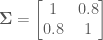
and covariance

In order to sample from this distribution using a Gibbs sampler, we need to have in hand the conditional distributions for variables/dimensions and :

(i.e. the conditional for the first dimension, )

and

(the conditional for the second dimension, )

Where is the previous state of the second dimension, and is the state of the first dimension after drawing from . The reason for the discrepancy between updating and using states and , can be is seen in step 3 of the algorithm outlined in the previous section. At iteration we first sample a new state for variable conditioned on the most recent state of variable , which is from iteration . We then sample a new state for the variable conditioned on the most recent state of variable , which is now from the current iteration, .

After some math (which which I will skip for some brevity, but see the following for some details), we find that the two conditional distributions for the target Normal distribution are:

and

,

which are both univariate Normal distributions, each with a mean that is dependent on the value of the most recent state of the conditioning variable, and a variance that is dependent on the target covariances between the two variables.

Using the above expressions for the conditional probabilities of variables and , we implement the Gibbs sampler using MATLAB below. The output of the sampler is shown here:

Gibbs sampler Markov chain and samples for bivariate Normal target distribution

Inspecting the figure above, note how at each iteration the Markov chain for the Gibbs sampler first takes a step only along the direction, then only along the direction.  This shows how the Gibbs sampler sequentially samples the value of each variable separately, in a component-wise fashion.

% EXAMPLE: GIBBS SAMPLER FOR BIVARIATE NORMAL
rand('seed' ,12345);
nSamples = 5000;

mu = [0 0]; % TARGET MEAN
rho(1) = 0.8; % rho_21
rho(2) = 0.8; % rho_12

% INITIALIZE THE GIBBS SAMPLER
propSigma = 1; % PROPOSAL VARIANCE
minn = [-3 -3];
maxx = [3 3];

% INITIALIZE SAMPLES
x = zeros(nSamples,2);
x(1,1) = unifrnd(minn(1), maxx(1));
x(1,2) = unifrnd(minn(2), maxx(2));

dims = 1:2; % INDEX INTO EACH DIMENSION

% RUN GIBBS SAMPLER
t = 1;
while t < nSamples
    t = t + 1;
    T = [t-1,t];
    for iD = 1:2 % LOOP OVER DIMENSIONS
        % UPDATE SAMPLES
        nIx = dims~=iD; % *NOT* THE CURRENT DIMENSION
        % CONDITIONAL MEAN
        muCond = mu(iD) + rho(iD)*(x(T(iD),nIx)-mu(nIx));
        % CONDITIONAL VARIANCE
        varCond = sqrt(1-rho(iD)^2);
        % DRAW FROM CONDITIONAL
        x(t,iD) = normrnd(muCond,varCond);
    end
end

% DISPLAY SAMPLING DYNAMICS
figure;
h1 = scatter(x(:,1),x(:,2),'r.');

% CONDITIONAL STEPS/SAMPLES
hold on;
for t = 1:50
    plot([x(t,1),x(t+1,1)],[x(t,2),x(t,2)],'k-');
    plot([x(t+1,1),x(t+1,1)],[x(t,2),x(t+1,2)],'k-');
    h2 = plot(x(t+1,1),x(t+1,2),'ko');
end

h3 = scatter(x(1,1),x(1,2),'go','Linewidth',3);
legend([h1,h2,h3],{'Samples','1st 50 Samples','x(t=0)'},'Location','Northwest')
hold off;
xlabel('x_1');
ylabel('x_2');
axis square

Wrapping Up

The Gibbs sampler is a popular MCMC method for sampling from complex, multivariate probability distributions. However, the Gibbs sampler cannot be used for general sampling problems. For many target distributions, it may difficult or impossible to obtain a closed-form expression for all the needed conditional distributions. In other scenarios, analytic expressions may exist for all conditionals but it may be difficult to sample from any or all of the conditional distributions (in these scenarios it is common to use univariate sampling methods such as rejection sampling and (surprise!) Metropolis-type MCMC techniques to approximate samples from each conditional). Gibbs samplers are very popular for Bayesian methods where models are often devised in such a way that conditional expressions for all model variables are easily obtained and take well-known forms that can be sampled from efficiently.

Gibbs sampling, like many MCMC techniques suffer from what is often called “slow mixing.” Slow mixing occurs when the underlying Markov chain takes a long time to sufficiently explore the values of in order to give a good characterization of . Slow mixing is due to a number of factors including the “random walk” nature of the Markov chain, as well as the tendency of the Markov chain to get “stuck,” only sampling a single region of having high-probability under . Such behaviors are bad for sampling distributions with multiple modes or heavy tails. More advanced techniques, such as Hybrid Monte Carlo have been developed to incorporate additional dynamics that increase the efficiency of the Markov chain path. We will discuss Hybrid Monte Carlo in a future post.

MCMC: Multivariate Distributions, Block-wise, & Component-wise Updates

In the previous posts on MCMC methods, we focused on how to sample from univariate target distributions. This was done mainly to give the reader some intuition about MCMC implementations with fairly tangible examples that can be visualized. However, MCMC can easily be extended to sample multivariate distributions.

In this post we will discuss two flavors of MCMC update procedure for sampling distributions in multiple dimensions: block-wise, and component-wise update procedures. We will show how these two different procedures can give rise to different implementations of the Metropolis-Hastings sampler to solve the same problem.

Block-wise Sampling

The first approach for performing multidimensional sampling is to use block-wise updates. In this approach the proposal distribution has the same dimensionality as the target distribution . Specifically, if is a distribution over variables, ie. , then we must design a proposal distribution that is also a distribution involving variables. We then accept or reject a proposed state sampled from the proposal distribution in exactly the same way as for the univariate Metropolis-Hastings algorithm. To generate multivariate samples we perform the following block-wise sampling procedure:

1. set
2. generate an initial state
3. repeat until

set

generate a proposal state from

calculate the proposal correction factor

calculate the acceptance probability

draw a random number from

if accept the proposal state and set

else set

Let’s take a look at the block-wise sampling routine in action.

Example 1: Block-wise Metropolis-Hastings for sampling of bivariate Normal distribution

In this example we use block-wise Metropolis-Hastings algorithm to sample from a bivariate (i.e. ) Normal distribution:

with mean

and covariance

Usually the target distribution will have a complex mathematical form, but for this example we’ll circumvent that by using MATLAB’s built-in function to evaluate . For our proposal distribution, , let’s use a circular Normal centered at the the previous state/sample of the Markov chain/sampler, i.e:

,

where is a 2-D identity matrix, giving the proposal distribution unit variance along both dimensions and , and zero covariance. You can find an MATLAB implementation of the block-wise sampler at the end of the section. The display of the samples and the target distribution output by the sampler implementation are shown below:

Samples drawn from block-wise Metropolis-Hastings sampler

We can see from the output that the block-wise sampler does a good job of drawing samples from the target distribution.

Note that our proposal distribution in this example is symmetric, therefore it was not necessary to calculate the correction factor per se. This means that this Metropolis-Hastings implementation is identical to the simpler Metropolis sampler.

%------------------------------------------------------
% EXAMPLE 1: METROPOLIS-HASTINGS
% BLOCK-WISE SAMPLER (BIVARIATE NORMAL)
rand('seed' ,12345);

D = 2; % # VARIABLES
nBurnIn = 100;

% TARGET DISTRIBUTION IS A 2D NORMAL WITH STRONG COVARIANCE
p = inline('mvnpdf(x,[0 0],[1 0.8;0.8 1])','x');

% PROPOSAL DISTRIBUTION STANDARD 2D GUASSIAN
q = inline('mvnpdf(x,mu)','x','mu')

nSamples = 5000;
minn = [-3 -3];
maxx = [3 3];

% INITIALIZE BLOCK-WISE SAMPLER
t = 1;
x = zeros(nSamples,2);
x(1,:) = randn(1,D);

% RUN SAMPLER
while t < nSamples
    t = t + 1;

    % SAMPLE FROM PROPOSAL
    xStar = mvnrnd(x(t-1,:),eye(D));

    % CORRECTION FACTOR (SHOULD EQUAL 1)
    c = q(x(t-1,:),xStar)/q(xStar,x(t-1,:));

    % CALCULATE THE M-H ACCEPTANCE PROBABILITY
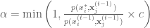
    alpha = min([1, p(xStar)/p(x(t-1,:))]);

    % ACCEPT OR REJECT?
    u = rand;
    if u < alpha
        x(t,:) = xStar;
    else
        x(t,:) = x(t-1,:);
    end
end

% DISPLAY
nBins = 20;
bins1 = linspace(minn(1), maxx(1), nBins);
bins2 = linspace(minn(2), maxx(2), nBins);

% DISPLAY SAMPLED DISTRIBUTION
ax = subplot(121);
bins1 = linspace(minn(1), maxx(1), nBins);
bins2 = linspace(minn(2), maxx(2), nBins);
sampX = hist3(x, 'Edges', {bins1, bins2});
hist3(x, 'Edges', {bins1, bins2});
view(-15,40)

% COLOR HISTOGRAM BARS ACCORDING TO HEIGHT
colormap hot
set(gcf,'renderer','opengl');
set(get(gca,'child'),'FaceColor','interp','CDataMode','auto');
xlabel('x_1'); ylabel('x_2'); zlabel('Frequency');
axis square
set(ax,'xTick',[minn(1),0,maxx(1)]);
set(ax,'yTick',[minn(2),0,maxx(2)]);
title('Sampled Distribution');

% DISPLAY ANALYTIC DENSITY
ax = subplot(122);
[x1 ,x2] = meshgrid(bins1,bins2);
probX = p([x1(:), x2(:)]);
probX = reshape(probX ,nBins, nBins);
surf(probX); axis xy
view(-15,40)
xlabel('x_1'); ylabel('x_2'); zlabel('p({\bfx})');
colormap hot
axis square
set(ax,'xTick',[1,round(nBins/2),nBins]);
set(ax,'xTickLabel',[minn(1),0,maxx(1)]);
set(ax,'yTick',[1,round(nBins/2),nBins]);
set(ax,'yTickLabel',[minn(2),0,maxx(2)]);
title('Analytic Distribution')

Component-wise Sampling

A problem with block-wise updates, particularly when the number of dimensions becomes large, is that finding a suitable proposal distribution is difficult. This leads to a large proportion of the samples being rejected. One way to remedy this is to simply loop over the the dimensions of in sequence, sampling each dimension independently from the others. This is what is known as using component-wise updates. Note that now the proposal distribution is univariate, working only in one dimension, namely the current dimension that we are trying to sample. The component-wise Metropolis-Hastings algorithm is outlined below.

1. set
2. generate an initial state
3. repeat until

set

for each dimension

generate a proposal state from

calculate the proposal correction factor 

calculate the acceptance probability

draw a random number from

if accept the proposal state  and set

else set

Note that in the component-wise implementation a sample for the -th dimension is proposed, then  accepted or rejected while all other dimensions () are held fixed. We then move on to the next (-th) dimension and repeat the process while holding all other variables () fixed. In each successive step we are using updated values for the dimensions that have occurred since increasing .

Example 2: Component-wise Metropolis-Hastings for sampling of bivariate Normal distribution

In this example we draw samples from the same bivariate Normal target distribution described in Example 1, but using component-wise updates. Therefore is the same, however, the proposal distribution is now a univariate Normal distribution with unit unit variance in the direction of the -th dimension to be sampled. The MATLAB implementation of the component-wise sampler is at the end of the section. The samples and comparison to the analytic target distribution are shown below.

Samples drawn from component-wise Metropolis-Hastings algorithm compared to target distribution

Again, we see that we get a good characterization of the bivariate target distribution.

%--------------------------------------------------
% EXAMPLE 2: METROPOLIS-HASTINGS
% COMPONENT-WISE SAMPLING OF BIVARIATE NORMAL
rand('seed' ,12345);

% TARGET DISTRIBUTION
p = inline('mvnpdf(x,[0 0],[1 0.8;0.8 1])','x');

nSamples = 5000;
propSigma = 1;		% PROPOSAL VARIANCE
minn = [-3 -3];
maxx = [3 3];

% INITIALIZE COMPONENT-WISE SAMPLER
x = zeros(nSamples,2);
xCurrent(1) = randn;
xCurrent(2) = randn;
dims = 1:2; % INDICES INTO EACH DIMENSION
t = 1;
x(t,1) = xCurrent(1);
x(t,2) = xCurrent(2);

% RUN SAMPLER
while t < nSamples
	t = t + 1;
	for iD = 1:2 % LOOP OVER DIMENSIONS

		% SAMPLE PROPOSAL
		xStar = normrnd(xCurrent(:,iD), propSigma);

		% NOTE: CORRECTION FACTOR c=1 BECAUSE
		% N(mu,1) IS SYMMETRIC, NO NEED TO CALCULATE

		% CALCULATE THE ACCEPTANCE PROBABILITY
		pratio = p([xStar xCurrent(dims~=iD)])/ ...
		p([xCurrent(1) xCurrent(2)]);
		alpha = min([1, pratio]);

		% ACCEPT OR REJECT?
		u = rand;
		if u < alpha
			xCurrent(iD) = xStar;
		end
	end

	% UPDATE SAMPLES
	x(t,:) = xCurrent;
end

% DISPLAY
nBins = 20;
bins1 = linspace(minn(1), maxx(1), nBins);
bins2 = linspace(minn(2), maxx(2), nBins);

% DISPLAY SAMPLED DISTRIBUTION
figure;
ax = subplot(121);
bins1 = linspace(minn(1), maxx(1), nBins);
bins2 = linspace(minn(2), maxx(2), nBins);
sampX = hist3(x, 'Edges', {bins1, bins2});
hist3(x, 'Edges', {bins1, bins2});
view(-15,40)

% COLOR HISTOGRAM BARS ACCORDING TO HEIGHT
colormap hot
set(gcf,'renderer','opengl');
set(get(gca,'child'),'FaceColor','interp','CDataMode','auto');
xlabel('x_1'); ylabel('x_2'); zlabel('Frequency');
axis square
set(ax,'xTick',[minn(1),0,maxx(1)]);
set(ax,'yTick',[minn(2),0,maxx(2)]);
title('Sampled Distribution');

% DISPLAY ANALYTIC DENSITY
ax = subplot(122);
[x1 ,x2] = meshgrid(bins1,bins2);
probX = p([x1(:), x2(:)]);
probX = reshape(probX ,nBins, nBins);
surf(probX); axis xy
view(-15,40)
xlabel('x_1'); ylabel('x_2'); zlabel('p({\bfx})');
colormap hot
axis square
set(ax,'xTick',[1,round(nBins/2),nBins]);
set(ax,'xTickLabel',[minn(1),0,maxx(1)]);
set(ax,'yTick',[1,round(nBins/2),nBins]);
set(ax,'yTickLabel',[minn(2),0,maxx(2)]);
title('Analytic Distribution')

Wrapping Up

Here we saw how we can use block- and component-wise updates to derive two different implementations of the Metropolis-Hastings algorithm. In the next post we will use component-wise updates introduced above to motivate the Gibbs sampler, which is often used to increase the efficiency of sampling well-defined probability multivariate distributions.

MCMC: The Metropolis-Hastings Sampler

In an earlier post we discussed how the Metropolis sampling algorithm can draw samples from a complex and/or unnormalized target probability distributions using a Markov chain. The Metropolis algorithm first proposes a possible new state in the Markov chain, based on a previous state , according to the proposal distribution . The algorithm accepts or rejects the proposed state based on the density of the the target distribution evaluated at . (If any of this Markov-speak is gibberish to the reader, please refer to the previous posts on Markov Chains, MCMC, and the Metropolis Algorithm for some clarification).

One constraint of the Metropolis sampler is that the proposal distribution must be symmetric. The constraint originates from using a Markov Chain to draw samples: a necessary condition for drawing from a Markov chain’s stationary distribution is that at any given point in time , the probability of moving from must be equal to the probability of moving from , a condition known as reversibility or detailed balance. However, a symmetric proposal distribution may be ill-fit for many problems, like when we want to sample from distributions that are bounded on semi infinite intervals (e.g. ).

In order to be able to use an asymmetric proposal distributions, the Metropolis-Hastings algorithm implements an additional correction factor , defined from the proposal distribution as

The correction factor adjusts the transition operator to ensure that the probability of moving from is equal to the probability of moving from , no matter the proposal distribution.

The Metropolis-Hastings algorithm is implemented with essentially the same procedure as the Metropolis sampler, except that the correction factor is used in the evaluation of acceptance probability .  Specifically, to draw samples using the Metropolis-Hastings sampler:

1. set t = 0
2. generate an initial state
3. repeat until

set

generate a proposal state from

calculate the proposal correction factor

calculate the acceptance probability

draw a random number from

if accept the proposal state and set

else set

Many consider the Metropolis-Hastings algorithm to be a generalization of the Metropolis algorithm. This is because when the proposal distribution is symmetric, the correction factor is equal to one, giving the transition operator for the Metropolis sampler.

Example: Sampling from a Bayesian posterior with improper prior

For a number of applications, including regression and density estimation, it is usually necessary to determine a set of parameters to an assumed model such that the model can best account for some observed data . The model function is often referred to as the likelihood function. In Bayesian methods there is often an explicit prior distribution that is placed on the model parameters and controls the values that the parameters can take.

The parameters are determined based on the posterior distribution , which is a probability distribution over the possible parameters based on the observed data. The posterior can be determined using Bayes’ theorem:

where, is a normalization constant that is often quite difficult to determine explicitly, as it involves computing sums over every possible value that the parameters and can take.

Let’s say that we assume the following model (likelihood function):

, where

, where

is the gamma function. Thus, the model parameters are

The parameter controls the shape of the distribution, and controls the scale. The likelihood surface for , and a number of values of ranging from zero to five are shown below.

Likelihood surface and conditional probability p(y|A=2,B=1) in green

 

The conditional distribution is plotted in green along the likelihood surface. You can verify this is a valid conditional in MATLAB with the following command:

 plot(0:.1:10,gampdf(0:.1:10,4,1)); % GAMMA(4,1)

Now, let’s assume the following priors on the model parameters:

and

The first prior states that only takes a single value (i.e. 1), therefore we can treat it as a constant. The second (rather non-conventional) prior states that the probability of varies as a sinusoidal function. (Note that both of these prior distributions are called improper priors because they do not integrate to one). Because is constant, we only need to estimate the value of .

It turns out that even though the normalization constant may be difficult to compute, we can sample from without knowing using the Metropolis-Hastings algorithm. In particular, we can ignore the normalization constant and sample from the unnormalized posterior:

The surface of the (unnormalized) posterior for ranging from zero to ten are shown below. The prior is displayed in blue on the right of the plot. Let’s say that we have a datapoint and would like to estimate the posterior distribution using the Metropolis-Hastings algorithm. This particular target distribution is plotted in magenta in the plot below.

Posterior surface, prior distribution (blue), and target distribution (pink)

Using a symmetric proposal distribution like the Normal distribution is not efficient for sampling from due to the fact that the posterior only has support on the real positive numbers . An asymmetric proposal distribution with the same support, would provide a better coverage of the posterior. One distribution that operates on the positive real numbers is the exponential distribution.

,

This distribution is parameterized by a single variable that controls the scale and location of the distribution probability mass. The target posterior and a proposal distribution (for ) are shown in the plot below.

Target posterior p(A|y) and proposal distribution q(A)

We see that the proposal has a fairly good coverage of the posterior distribution. We run the Metropolis-Hastings sampler in the block of MATLAB code at the bottom. The Markov chain path and the resulting samples are shown in plot below.

Metropolis-Hastings Markov chain and samples

As an aside, note that the proposal distribution for this sampler does not depend on past samples, but only on the parameter (see line 88 in the MATLAB code below). Each proposal states is drawn independently of the previous state. Therefore this is an example of an independence sampler, a specific type of Metropolis-Hastings sampling algorithm. Independence samplers are notorious for being either very good or very poor sampling routines. The quality of the routine depends on the choice of the proposal distribution, and its coverage of the target distribution. Identifying such a proposal distribution is often difficult in practice.

The MATLAB  code for running the Metropolis-Hastings sampler is below. Use the copy icon in the upper right of the code block to copy it to your clipboard. Paste in a MATLAB terminal to output the figures above.

% METROPOLIS-HASTINGS BAYESIAN POSTERIOR
rand('seed',12345)

% PRIOR OVER SCALE PARAMETERS
B = 1;

% DEFINE LIKELIHOOD
likelihood = inline('(B.^A/gamma(A)).*y.^(A-1).*exp(-(B.*y))','y','A','B');

% CALCULATE AND VISUALIZE THE LIKELIHOOD SURFACE
yy = linspace(0,10,100);
AA = linspace(0.1,5,100);
likeSurf = zeros(numel(yy),numel(AA));
for iA = 1:numel(AA); likeSurf(:,iA)=likelihood(yy(:),AA(iA),B); end;

figure;
surf(likeSurf); ylabel('p(y|A)'); xlabel('A'); colormap hot

% DISPLAY CONDITIONAL AT A = 2
hold on; ly = plot3(ones(1,numel(AA))*40,1:100,likeSurf(:,40),'g','linewidth',3)
xlim([0 100]); ylim([0 100]);  axis normal
set(gca,'XTick',[0,100]); set(gca,'XTickLabel',[0 5]);
set(gca,'YTick',[0,100]); set(gca,'YTickLabel',[0 10]);
view(65,25)
legend(ly,'p(y|A=2)','Location','Northeast');
hold off;
title('p(y|A)');

% DEFINE PRIOR OVER SHAPE PARAMETERS
prior = inline('sin(pi*A).^2','A');

% DEFINE THE POSTERIOR
p = inline('(B.^A/gamma(A)).*y.^(A-1).*exp(-(B.*y)).*sin(pi*A).^2','y','A','B');

% CALCULATE AND DISPLAY THE POSTERIOR SURFACE
postSurf = zeros(size(likeSurf));
for iA = 1:numel(AA); postSurf(:,iA)=p(yy(:),AA(iA),B); end;

figure
surf(postSurf); ylabel('y'); xlabel('A'); colormap hot

% DISPLAY THE PRIOR
hold on; pA = plot3(1:100,ones(1,numel(AA))*100,prior(AA),'b','linewidth',3)

% SAMPLE FROM p(A | y = 1.5)
y = 1.5;
target = postSurf(16,:);

% DISPLAY POSTERIOR
psA = plot3(1:100, ones(1,numel(AA))*16,postSurf(16,:),'m','linewidth',3)
xlim([0 100]); ylim([0 100]);  axis normal
set(gca,'XTick',[0,100]); set(gca,'XTickLabel',[0 5]);
set(gca,'YTick',[0,100]); set(gca,'YTickLabel',[0 10]);
view(65,25)
legend([pA,psA],{'p(A)','p(A|y = 1.5)'},'Location','Northeast');
hold off
title('p(A|y)');

% INITIALIZE THE METROPOLIS-HASTINGS SAMPLER
% DEFINE PROPOSAL DENSITY
q = inline('exppdf(x,mu)','x','mu');

% MEAN FOR PROPOSAL DENSITY
mu = 5;

% DISPLAY TARGET AND PROPOSAL
figure; hold on;
th = plot(AA,target,'m','Linewidth',2);
qh = plot(AA,q(AA,mu),'k','Linewidth',2)
legend([th,qh],{'Target, p(A)','Proposal, q(A)'});
xlabel('A');

% SOME CONSTANTS
nSamples = 5000;
burnIn = 500;
minn = 0.1; maxx = 5;

% INTIIALZE SAMPLER
x = zeros(1 ,nSamples);
x(1) = mu;
t = 1;

% RUN METROPOLIS-HASTINGS SAMPLER
while t < nSamples
	t = t+1;

	% SAMPLE FROM PROPOSAL
	xStar = exprnd(mu);

	% CORRECTION FACTOR
	c = q(x(t-1),mu)/q(xStar,mu);

	% CALCULATE THE (CORRECTED) ACCEPTANCE RATIO
	alpha = min([1, p(y,xStar,B)/p(y,x(t-1),B)*c]);

	% ACCEPT OR REJECT?
	u = rand;
	if u < alpha
		x(t) = xStar;
	else
		x(t) = x(t-1);
	end
end

% DISPLAY MARKOV CHAIN
figure;
subplot(211);
stairs(x(1:t),1:t, 'k');
hold on;
hb = plot([0 maxx/2],[burnIn burnIn],'g--','Linewidth',2)
ylabel('t'); xlabel('samples, A');
set(gca , 'YDir', 'reverse');
ylim([0 t])
axis tight;
xlim([0 maxx]);
title('Markov Chain Path');
legend(hb,'Burnin');

% DISPLAY SAMPLES
subplot(212);
nBins = 100;
sampleBins = linspace(minn,maxx,nBins);
counts = hist(x(burnIn:end), sampleBins);
bar(sampleBins, counts/sum(counts), 'k');
xlabel('samples, A' ); ylabel( 'p(A | y)' );
title('Samples');
xlim([0 10])

% OVERLAY TARGET DISTRIBUTION
hold on;
plot(AA, target/sum(target) , 'm-', 'LineWidth', 2);
legend('Sampled Distribution',sprintf('Target Posterior'))
axis tight

Wrapping Up

Here we explored how the Metorpolis-Hastings sampling algorithm can be used to generalize the Metropolis algorithm in order to sample from complex (an unnormalized) probability distributions using asymmetric proposal distributions. One shortcoming of the Metropolis-Hastings algorithm is that not all of the proposed samples are accepted, wasting valuable computational resources. This becomes even more of an issue for sampling distributions in higher dimensions. This is where Gibbs sampling comes in. We’ll see in a later post that Gibbs sampling can be used to keep all proposal states in the Markov chain by taking advantage of conditional probabilities.

MCMC: The Metropolis Sampler

As discussed in an earlier post, we can use a Markov chain to sample from some target probability distribution from which drawing samples directly is difficult. To do so, it is necessary to design a transition operator for the Markov chain which makes the chain’s stationary distribution match the target distribution. The Metropolis sampling algorithm  (and the more general Metropolis-Hastings sampling algorithm) uses simple heuristics to implement such a transition operator.

Metropolis Sampling

Starting from some random initial state , the algorithm first draws a possible sample from a  proposal distribution .  Much like a conventional transition operator for a Markov chain, the proposal distribution depends only on the previous state in the chain. However, the transition operator for the Metropolis algorithm has an additional step that assesses whether or not the target distribution has a sufficiently large density near the proposed state to warrant accepting the proposed state as a sample and setting it to the next state in the chain. If the density of is low near the proposed state, then it is likely (but not guaranteed) that it will be rejected. The criterion for accepting or rejecting a proposed state are defined by the following heuristics:

1. If ,  the proposed state is kept as a sample and is set as the next state in the chain (i.e. move the chain’s state to a location  where has equal or greater density).
2. If –indicating that has low density near –then the proposed state may still be accepted, but only randomly, and with a probability

These heuristics can be instantiated by calculating the acceptance probability for the proposed state.

Having the acceptance probability in hand, the transition operator for the metropolis algorithm works like this: if a random uniform number is less than or equal to , then the state is accepted (as in (1) above), if not, it is rejected and another state is proposed (as in (2) above). In order to collect samples using  Metropolis sampling we run the following algorithm:

1. set t = 0
2. generate an initial state from a prior distribution over initial states
3. repeat until

set

generate a proposal state from

calculate the acceptance probability 

draw a random number from

if , accept the proposal and set

else  set

Example: Using the Metropolis algorithm to sample from an unknown distribution

Say that we have some mysterious function

from which we would like to draw samples. To do so using Metropolis sampling we need to define two things: (1) the prior distribution over the initial state of the Markov chain, and (2)  the proposal distribution . For this example we define:

,

both of which are simply a Normal distribution, one centered at zero, the other centered at previous state of the chain. The following chunk of MATLAB code runs the Metropolis sampler with this proposal distribution and prior.

% METROPOLIS SAMPLING EXAMPLE
randn('seed',12345);

% DEFINE THE TARGET DISTRIBUTION
p = inline('(1 + x.^2).^-1','x')

% SOME CONSTANTS
nSamples = 5000;
burnIn = 500;
nDisplay = 30;
sigma = 1;
minn = -20; maxx = 20;
xx = 3*minn:.1:3*maxx;
target = p(xx);
pauseDur = .8;

% INITIALZE SAMPLER
x = zeros(1 ,nSamples);
x(1) = randn;
t = 1;

% RUN SAMPLER
while t < nSamples
	t = t+1;

	% SAMPLE FROM PROPOSAL
	xStar = normrnd(x(t-1) ,sigma);
	proposal = normpdf(xx,x(t-1),sigma);

	% CALCULATE THE ACCEPTANCE PROBABILITY
	alpha = min([1, p(xStar)/p(x(t-1))]);

	% ACCEPT OR REJECT?
	u = rand;
	if u < alpha
		x(t) = xStar;
		str = 'Accepted';
	else
		x(t) = x(t-1);
		str = 'Rejected';
	end

	% DISPLAY SAMPLING DYNAMICS
	if t < nDisplay + 1
		figure(1);
		subplot(211);
		cla
		plot(xx,target,'k');
		hold on;
		plot(xx,proposal,'r');
		line([x(t-1),x(t-1)],[0 p(x(t-1))],'color','b','linewidth',2)
		scatter(xStar,0,'ro','Linewidth',2)
		line([xStar,xStar],[0 p(xStar)],'color','r','Linewidth',2)
		plot(x(1:t),zeros(1,t),'ko')
		legend({'Target','Proposal','p(x^{(t-1)})','x^*','p(x^*)','Kept Samples'})

		switch str
			case 'Rejected'
				scatter(xStar,p(xStar),'rx','Linewidth',3)
			case 'Accepted'
				scatter(xStar,p(xStar),'rs','Linewidth',3)
		end
           	scatter(x(t-1),p(x(t-1)),'bo','Linewidth',3)
		title(sprintf('Sample % d %s',t,str))
		xlim([minn,maxx])
		subplot(212);
		hist(x(1:t),50); colormap hot;
		xlim([minn,maxx])
		title(['Sample ',str]);
		drawnow
		pause(pauseDur);
	end
end

% DISPLAY MARKOV CHAIN
figure(1); clf
subplot(211);
stairs(x(1:t),1:t, 'k');
hold on;
hb = plot([-10 10],[burnIn burnIn],'b--')
ylabel('t'); xlabel('samples, x');
set(gca , 'YDir', 'reverse');
ylim([0 t])
axis tight;
xlim([-10 10]);
title('Markov Chain Path');
legend(hb,'Burnin');

% DISPLAY SAMPLES
subplot(212);
nBins = 200;
sampleBins = linspace(minn,maxx,nBins);
counts = hist(x(burnIn:end), sampleBins);
bar(sampleBins, counts/sum(counts), 'k');
xlabel('samples, x' ); ylabel( 'p(x)' );
title('Samples');

% OVERLAY ANALYTIC DENSITY OF STUDENT T
nu = 1;
y = tpdf(sampleBins,nu)
hold on;
plot(sampleBins, y/sum(y) , 'r-', 'LineWidth', 2);
legend('Samples',sprintf('Theoretic\nStudent''s t'))
axis tight
xlim([-10 10]);

Using the Metropolis algorithm to sample from a continuous distribution (black)

In the figure above, we visualize the first 50 iterations of the Metropolis sampler.The black curve represents the target distribution . The red curve that is bouncing about the x-axis is the proposal distribution (if the figure is not animated, just click on it). The vertical blue line (about which the bouncing proposal distribution is centered) represents the quantity , and the vertical red line represents the quantity , for a proposal state sampled according to the red  curve. At every iteration, if the vertical red line is longer than the blue line, then the sample is accepted, and the proposal distribution becomes centered about the newly accepted sample. If the blue line is longer, the sample is randomly rejected or accepted.

But why randomly keep “bad” proposal samples? It turns out that doing this allows the Markov chain to every-so-often visit states of low probability under the target distribution. This is a desirable property if we want the chain to adequately sample the entire target distribution, including any tails.

An attractive property of the Metropolis algorithm is that the target distribution does not have to be a properly normalized probability distribution. This is due to the fact that the acceptance probability is based on the ratio of two values of the target distribution. I’ll show you what I mean. If is an unnormalized distribution and

is a properly normalized probability distribution with normalizing constant , then

and a ratio like that used in calculating the acceptance probability is

The normalizing constants cancel! This attractive property is quite useful in the context of Bayesian methods, where determining the normalizing constant for a distribution may be impractical to calculate directly. This property is demonstrated in current example. It turns out that the “mystery” distribution that we sampled from using the Metropolis algorithm is an unnormalized form of the Student’s-t distribution with one degree of freedom. Comparing to the definition of the definition Student’s-t

we see that is a Student’s-t distribution with degrees of freedom , but missing the normalizing constant

Below is additional output from the code above showing that the samples from Metropolis sampler draws samples that follow a normalized Student’s-t distribution, even though is not normalized.

Metropolis samples from an unnormalized t-distribution follow the normalized distribution

The upper plot shows the progression of the Markov chain’s progression from state (top) to state (bottom). The burn in period for this chain was chosen to be 500 transitions, and is indicated by the dashed blue line (for more on burnin see this previous post).

The bottom plot shows samples from the Markov chain in black (with burn in samples removed). The theoretical curve for the Student’s-t with one degree of freedom is overlayed in red. We see that the states kept by the Metropolis sampler transition operator sample from values that follow the Student’s-t, even though the function used in the transition operator was not a properly normalized probability distribution.

Reversibility of the transition operator

It turns out that there is a theoretical constraint on the Markov chain the transition operator in order for it settle into a stationary distribution (i.e. a target distribution we care about). The constraint states that the probability of the transition must be equal to the probability of the reverse transition . This reversibility property is often referred to as detailed balance. Using the Metropolis algorithm transition operator, reversibility is assured if the proposal distribution is symmetric. Such symmetric proposal distributions are the Normal, Cauchy, Student’s-t, and Uniform distributions.

However, using a symmetric proposal distribution may not be reasonable to adequately or efficiently sample all possible target distributions. For instance if a target distribution is bounded on the positive numbers , we would like to use a proposal distribution that has the same support, and will thus be assymetric. This is where the Metropolis-Hastings sampling algorithm comes in. We will discuss in a later post how the Metropolis-Hastings sampler uses a simple change to the calculation of the acceptance probability which allows us to use non-symmetric proposal distributions.

A Brief Introduction to Markov Chains

Markov chains are an essential component of Markov chain Monte Carlo (MCMC) techniques. Under MCMC, the Markov chain is used to sample from some target distribution. To get a better understanding of what a Markov chain is, and further, how it can be used to sample form a distribution, this post introduces and applies a few basic concepts.

A Markov chain is a stochastic process that operates sequentially (e.g. temporally), transitioning from one state to another within an allowed set of states.^†

A Markov chain is defined by three elements:

1. A state space , which is a set of values that the chain is allowed to take
2. A transition operator that defines  the probability of moving from state to  .
3. An initial condition distribution which defines the probability of being in any one of the possible states at the initial iteration .

The Markov chain starts at some initial state, which is sampled from , then transitions from one state to another according to the transition operator .

A Markov chain is called memoryless if the next state only depends on the current state and not on any of the states previous to the current:

(This memoryless property is formally know as the Markov property).

If the transition operator for a Markov chain does not change across transitions, the Markov chain is called time homogenous.  A nice  property of time homogenous Markov chains is that as the chain runs for a long time and , the chain will reach an equilibrium that is called the chain’s stationary distribution:

We’ll see later how the stationary distribution of a Markov chain is important for sampling from probability distributions, a technique that is at the heart of Markov Chain Monte Carlo (MCMC) methods.

Finite state-space (time homogenous) Markov chain

If the state space of a Markov chain takes on a finite number of distinct values, and it is time homogenous, then the transition operator can be defined by a matrix , where the entries of are:

This means that if the chain is currently in the -th state, the transition operator assigns the probability of moving to the  -th state by the entries of -th row of (i.e.  each row of defines a conditional probability distribution on the state space). Let’s take a look at a finite state-space Markov chain in action with a simple example.

Example: Predicting the weather with a finite state-space Markov chain

In Berkeley, CA, there are (literally) only 3 types of weather: sunny, foggy, or rainy (this is analogous to a state-space that takes on three discrete values). The weather patterns are very stable there, so a Berkeley weatherman can easily predict the weather next week based on the weather today with the following transition rules:

If it is sunny today, then

• it is highly likely that it will be sunny next week
  • ,
• it is very unlikely that it will be raining next week
  • 
• and somewhat likely that it will foggy next week
  • 

If it is foggy today then

• it is somewhat likely that it will be sunny next week
  • 
• but slightly less likely that it will be foggy next week
  • ,
• and fairly unlikely that it will be raining next week.
  • ,

If it is rainy today then

• it is unlikely that it will be sunny next week
  • ,
• it is somewhat likely that it will be foggy next week
  • ,
• and it is fairly likely that it will be rainy next week
  • ,

All of these transition rules can be instantiated in a single 3 x 3 transition operator matrix:

Where each row of corresponds to the weather at iteration (today), and each column corresponds to the weather the next week. Let’s say that it is rainy today, what is the probability it will be sunny next week, in two weeks, or in 6 months? We can answer these questions by running a Markov chain from the initial state of “rainy,” transitioning according to . The following chunk of MATLAB code runs the Markov chain.

% FINITE STATE-SPACE MARKOV CHAIN EXAMPLE

% TRANSITION OPERATOR
%     S  F  R
%     U  O  A
%     N  G  I
%     N  G  N
%     Y  Y  Y
P = [.8 .15 .05;  % SUNNY
     .4 .5  .1;   % FOGGY
     .1 .3  .6];  % RAINY
nWeeks = 25

% INITIAL STATE IS RAINY
X(1,:) = [0 0 1];

% RUN MARKOV CHAIN
for iB = 2:nWeeks
    X(iB,:) = X(iB-1,:)*P; % TRANSITION
end

% DISPLAY
figure; hold on
h(1) = plot(1:nWeeks,X(:,1),'r','Linewidth',2);
h(2) = plot(1:nWeeks,X(:,2),'k','Linewidth',2);
h(3) = plot(1:nWeeks,X(:,3),'b','Linewidth',2);
h(4) = plot([15 15],[0 1],'g--','Linewidth',2);
hold off
legend(h, {'Sunny','Foggy','Rainy','Burn In'});
xlabel('Week')
ylabel('p(Weather)')
xlim([1,nWeeks]);
ylim([0 1]);

% PREDICTIONS
fprintf('\np(weather) in 1 week -->'), disp(X(2,:))
fprintf('\np(weather) in 2 weeks -->'), disp(X(3,:))
fprintf('\np(weather) in 6 months -->'), disp(X(25,:))

Finite state-space Markov chain for predicting the weather

Here we see that at week 1 the probability of sunny weather is 0.1. The next week, the probability of sunny weather is 0.26, and in 6 months, there is a 60% chance that it will be sunny. Also note that after approximately 15 weeks the Markov chain has reached the equilibrium/stationary distribution and, chances are, the weather will be sunny. This 15-week period is what is known as the burn in period for the Markov chain, and is the number of transitions it takes the chain to move from the initial conditions to the stationary distribution.

A cool thing about finite state-space time-homogeneous Markov chain is that it is not necessary  to run the chain sequentially through all iterations in order to predict a state in the future. Instead we can predict by first raising the transition operator to the -th power, where is the iteration at which we want to predict, then multiplying the result by the distribution over the initial state, . For instance, to predict the probability of the weather in 2 weeks, knowing that it is rainy today (i.e. ):

and in six months:

These are the same results we get by running the Markov chain sequentially through each number of transitions. Therefore we can calculate an approximation to the stationary distribution from by setting to a large number. It turns out that it is also possible to analytically derive the stationary distribution from (hint: think about the properties of eigenvectors).

Continuous state-space Markov chains

A Markov chain can also have a continuous state space that exists in the real numbers . In this case the transition operator cannot be instantiated simply as a matrix, but is instead some continuous function on the real numbers. Note that the continuous state-space Markov chain also has a burn in period and a stationary distribution. However, the stationary distribution will also be over a continuous set of variables. To get a better understanding of the workings of a continuous state-space Markov chain, let’s look at a simple example.

Example: Sampling from a continuous distribution using continuous state-space Markov chains

We can use the stationary distribution of a continuous state-space Markov chain in order to sample from a continuous probability distribution: we  run a Markov chain for a sufficient amount of time so that it has reached its stationary distribution, then keep the states that the chain visits as samples from that stationary distribution.

In the following example we define a continuous state-space Markov chain. The transition operator is a Normal distribution with unit variance and a mean that is half the distance between zero and the previous state, and the distribution over initial conditions is a Normal distribution with zero mean and unit variance.

To ensure that the chain has moved sufficiently far from the initial conditions and that we are sampling  from the chain’s stationary distribution,  we will choose to throw away the first 50 burn in states of the chain. We can also run multiple chains simultaneously in order to sample the stationary distribution more densely. Here we choose to run 5 chains simultaneously.

% EXAMPLE OF CONTINUOUS STATE-SPACE MARKOV CHAIN

% INITIALIZE
randn('seed',12345)
nBurnin = 50; % # BURNIN
nChains = 5;  % # MARKOV CHAINS

% DEFINE TRANSITION OPERATOR
P = inline('normrnd(.5*x,1,1,nChains)','x','nChains');
nTransitions = 1000;
x = zeros(nTransitions,nChains);
x(1,:) = randn(1,nChains);

% RUN THE CHAINS
for iT = 2:nTransitions
    x(iT,:) = P(x(iT-1),nChains);
end

% DISPLAY BURNIN
figure
subplot(221); plot(x(1:100,:)); hold on;
minn = min(x(:));
maxx = max(x(:));
l = line([nBurnin nBurnin],[minn maxx],'color','k','Linewidth',2);
ylim([minn maxx])
legend(l,'~Burn-in','Location','SouthEast')
title('First 100 Samples'); hold off

% DISPLAY ENTIRE MARKOV CHAIN
subplot(223); plot(x);hold on;
l = line([nBurnin nBurnin],[minn maxx],'color','k','Linewidth',2);
legend(l,'~Burn-in','Location','SouthEast')
title('Entire Chain');

% DISPLAY SAMPLES FROM STATIONARY DISTRIBUTION
samples = x(nBurnin+1:end,:);
subplot(122);
[counts,bins] = hist(samples(:),100); colormap hot
b = bar(bins,counts);
legend(b,sprintf('Markov Chain\nSamples'));
title(['\mu=',num2str(mean(samples(:))),' \sigma=',num2str(var(samples(:)))])

Sampling from the stationary distribution of a continuous state-space Markov chain

In the upper left panel of the code output we see a close up of the first 100 of the 1000 transitions made by the 5 simultaneous Markov chains; the burn in cutoff is marked by the black line. In the lower left panel we see the entire sequence of transitions for the Markov chains. In the right panel, we can tell from the sampled states that the stationary distribution for this chain is a Normal distribution, with mean equal to zero, and a variance equal to 1.3.

Wrapping Up

In the previous example we were able to deduce the stationary distribution of the Markov chain by looking at the samples generated from the chain after the burn in period. However, in order to use Markov chains to sample from a specific target distribution, we have to design the transition operator such that the resulting chain reaches a stationary distribution that matches the target distribution. This is where MCMC methods like the Metropolis sampler, the Metropolis-Hastings sampler, and the Gibbs sampler come to rescue. We will discuss each of these Markov-chain-based sampling methods separately in later posts.

Monte Carlo Approximations

Monte Carlo Approximation for Integration

Using statistical methods we often run into integrals that take the form:

For instance, the expected value of a some function of a random variable

and many quantities essential for Bayesian methods such as the marginal likelihood a.k.a “model evidence”

involve integrals of this form.  Sometimes (not often) such an integral can be evaluated analytically. When a closed form solution does not exist, numeric integration methods can be applied. However numerical methods quickly become intractable for any practical application that requires more than a small number of dimensions. This is where Monte Carlo approximation comes in. Monte Carlo approximation allows us to calculate an estimate for the value of by transforming the  integration problem into a procedure of sampling values from a tractable probability distribution and calculating the average of those samples. Here’s what I mean:

If the function fullfills two simple criteria, namely that the function is always positive on the interval

and that the integral of the function is finite

then we can define a corresponding probability distribution on the interval :

Another way to think of it is that is a probability distribution scaled by a constant .

Using this link between probability distributions and , we can restate the original integration as

This statement says that if we can sample values of using , then the value of  the original integral is simply a scaled version of the expected value of the integrand function calculated using those samples. Turns out that the expected value can be easily approximated by the sample mean:

where samples are drawn independently from . This leads to a simple 4-Step Procedure for performing Monte Carlo approximation to the integral :

1. Identify
2. Identify and from it determine and
3. Draw independent samples from
4. Evaluate

The larger the number of samples we draw, the better our approximation to the actual value of . This 4-step procedure is demonstrated in a some toy examples below:

Example 1: Approximating the integral

Say we want to calculate the integral:

We can calculate the closed form solution of this integral using integration by parts:

and

Orr…we could calculate the  Monte Carlo approximation of this integral.

Step 1 we identify

Step 2 we identify

and from this can also determine the probability distribution function . According to the definition expression for given above we detemine to be:

.

Step 3: The expression on the right is the definition for the uniform distribution , which is easy to sample from using the MATLAB (Notice too that the constant ).

Step 4: we calculate the Monte Carlo approximation as

,

where each is sampled from the standard uniform distribution. Below is some MATLAB code running the Monte Carlo Approximation for two different values of

% MONTE CARLO APPROXIMATION OF INT(xexp(x))dx
% FOR TWO DIFFERENT SAMPLE SIZES
rand('seed',12345);

% THE FIRST APPROXIMATION USING N1 = 100 SAMPLES
N1 = 100;
x = rand(N1,1);
Ihat1 = sum(x.*exp(x))/N1

% A SECOND APPROXIMATION USING N2 = 5000 SAMPLES
N2 = 5000;
x = rand(N2,1);
Ihat2 = sum(x.*exp(x))/N2

Comparing the values of the variables and we see that the Monte Carlo approximation is better for a larger number of samples.

Example 2: Approximating the expected value of the Beta distribution

Lets look at how the 4-step Monte Carlo approximation procedure can be used to calculate expectations. In this example we will calculate

,

where .

Step 1: we identify .

Step 2: the function is simply the probability density function due the expression for above:

.

Step 3 we can use MATLAB to easily draw independent samples using the function . And finally,

Step 4 we approximate the expectation with the expression

Below is some MATLAB code that performs this approximation of the expected value.

rand('seed',12345);
alpha1 = 2; alpha2 = 10;
N = 10000;
x = betarnd(alpha1,alpha2,1,N);

% MONTE CARLO EXPECTATION
expectMC = mean(x);

% ANALYTIC EXPRESSION FOR BETA MEAN
expectAnalytic = alpha1/(alpha1 + alpha2);

% DISPLAY
figure;
bins = linspace(0,1,50);
counts = histc(x,bins);
probSampled = counts/sum(counts);
probTheory = betapdf(bins,alpha1,alpha2);
b = bar(bins,probSampled); colormap hot; hold on;
t = plot(bins,probTheory/sum(probTheory),'r','Linewidth',2)
m = plot([expectMC,expectMC],[0 .1],'g')
e = plot([expectAnalytic,expectAnalytic],[0 .1],'b')
xlim([expectAnalytic - .05,expectAnalytic + 0.05])
legend([b,t,m,e],{'Samples','Theory','$\hat{E}$','$E_{Theory}$'},'interpreter','latex');
title(['E_{MC} = ',num2str(expectMC),'; E_{Theory} = ',num2str(expectAnalytic)])
hold off

And the output of the code:

Monte Carlo Approximation of the the Expected value of Beta(2,10)

The analytical solution for the expected value of this Beta distribution:

is quite close to our approximation (also indicated by the small distance between the blue and green lines on the plot above).

Monte Carlo Approximation for Optimization

Monte Carlo Approximation can also be used to solve optimization problems of the form:

If fulfills the same criteria described above (namely that it is a scaled version of a probability distribution), then (as above) we can define the probability function

This allows us to instead solve the problem

If we can sample from , the solution is easily found by drawing samples from and determining the location of the samples that has the highest density (Note that the solution is not dependent of the value of ). The following example demonstrates Monte Carlo optimization:

Example: Monte Carlo Optimization of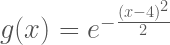

Say we would like to find the value of which optimizes the function . In other words we want to solve the problem

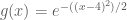
We could solve for using standard calculus methods, but a clever trick is to use Monte Carlo approximation to solve the problem. First, notice that  is  a scaled version of a Normal distribution with mean equal to 4 and unit variance:

where . This means we can solve for by drawing samples from the normal distribution and determining where those samples have the highest density. The following chunk of matlab code solves the optimization problem in this way.

% MONTE CARLO OPTIMIZATION OF exp(x-4)^2
randn('seed',12345)

% INITIALZIE
N = 100000;
x = 0:.1:6;
C = sqrt(2*pi);
g = inline('exp(-.5*(x-4).^2)','x');
ph = plot(x,g(x)/C,'r','Linewidth',3); hold on
gh = plot(x,g(x),'b','Linewidth',2); hold on;
y = normpdf(x,4,1);

% CALCULATE MONTE CARLO APPROXIMATION
x = normrnd(4,1,1,N);
bins = linspace(min(x),max(x),100);
counts = histc(x,bins);
[~,optIdx] = max(counts);
xHat = bins(optIdx);

% OPTIMA AND ESTIMATED OPTIMA
oh = plot([4 4],[0,1],'k');
hh = plot([xHat,xHat],[0,1],'g');

set(gca,'fontsize',16)
legend([gh,ph,oh,hh],{'g(x)','$p(x)=\frac{g(x)}{C}$','$x_{opt}$','$\hat{x}$'},'interpreter','latex','Location','Northwest');

Monte Carlo Optimization

In the code output above we see the function we want to optimize in blue and the Normal distribution from which we draw samples in red. The Monte Carlo method provides a good approximation (green) to the real solution (black).

Wrapping Up

In the toy examples above it was easy to sample from . However, for practical problems the distributions we want to sample from are often complex and operate in many dimensions. For these problems more clever sampling methods have to be used. Such sampling methods include Inverse Transform Sampling, Rejection Sampling, Importance Sampling, and Markov Chain Monte Carlo methods such as the Metropolis Hasting algorithm and the Gibbs sampler, each of which I plan to cover in separate posts.

Sampling From the Normal Distribution Using the Box-Muller Transform

The Normal Distribution is the workhorse of many common statistical analyses and being able to draw samples from this distribution lies at the heart of many statistical/machine learning algorithms. There have been a number of methods developed to sample from the Normal distribution including Inverse Transform Sampling, the Ziggurat Algorithm, and the Ratio Method (a rejection sampling technique). In this post we will focus on an elegant method called the Box-Muller transform.

A quick review of Cartesian and polar coordinates.

Before we can talk about using the Box-Muller transform, let’s refresh our understanding of the relationship between Cartesian and polar coordinates. You may remember from geometry that if x and y are two points in the Cartesian plane they can be represented in polar coordinates with a radius and an angle using the following relationships:

, and therefore

Notice that if and , then we map out values contained in the unit circle, as shown in the figure below. Also note that random variables in such a circle can be generated by transforming values sampled from the uniform distribution. Specifically, radii can be sampled from and angle can be sampled from . A similar mechanism (i.e. drawing points in a circle using uniform variables) is at the heart of the Box-Muller transform for sampling Normal random variables.

Example of the relationship between Cartesian and polar coordinates

Drawing Normally-distributed samples with the Box-Muller transform

Ok, now that we’ve discussed how Cartesian coordinates are represented in polar coordinates, let’s move on to how we can use this relationship to generate random variables. Box-Muller sampling is based on representing the joint distribution of two independent standard Normal random Cartesian variables and

in polar coordinates. The joint distribution (which is circular-symmetric) is:

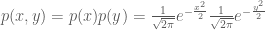
If we notice that the term in the numerator of the exponent is equal to (as above) we can make the connection between the the Cartesian representation of the joint Normal distribution and its polar representation:

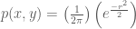
which is the product of two density functions, an exponential distribution over squared radii:

and a uniform distribution over angles:

just like those mentioned above when generating points on the unit circle. Now, if we make another connection between the exponential distribution and the uniform distribution, namely that:

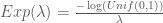
then

This gives us a way to generate points from the joint Gaussian distribution by sampling from two independent uniform distributions, one for and another for , and transforming them into Cartesian coordinates via the relationships above. In detail, the procedure goes as follows:

1. Draw,
2. Transform the variables into radius and angle representation , and
3. Transform radius and angle into Cartesian coordinates:

What results are two independent Normal random variables, and . A MATLAB implementation of the Box-Muller algorithm is shown below:

% NORMAL SAMPLES USING BOX-MUELLER METHOD
% DRAW SAMPLES FROM PROPOSAL DISTRIBUTION
u = rand(2,100000);
r = sqrt(-2*log(u(1,:)));
theta = 2*pi*u(2,:);
x = r.*cos(theta);
y = r.*sin(theta);

% DISPLAY BOX-MULLER SAMPLES
figure
% X SAMPLES
subplot(121);
hist(x,100);
colormap hot;axis square
title(sprintf('Box-Muller Samples Y\n Mean = %1.2f\n Variance = %1.2f\n Kurtosis = %1.2f',mean(x),var(x),3-kurtosis(x)))
xlim([-6 6])

% Y SAMPLES
subplot(122);
hist(y,100);
colormap hot;axis square
title(sprintf('Box-Muller Samples X\n Mean = %1.2f\n Variance = %1.2f\n Kurtosis = %1.2f',mean(y),var(y),3-kurtosis(y)))
xlim([-6 6])

Box-Muller Samples for Normal Distribution

Wrapping Up

The output of the MATLAB code is shown above. Notice the first, second, and fourth central moments (mean, variance, and kurtosis)  of the generated samples are consistent with the standard normal. The Box-Muller transform is another example of of how uniform variables on the interval (0,1) and can be  transformed in order to sample from a more complicated distribution.

Rejection Sampling

Suppose that we want to sample from a distribution that is difficult or impossible to sample from directly, but instead have a simpler distribution from which sampling is easy.  The idea behind Rejection sampling (aka Acceptance-rejection sampling) is to sample from and apply some rejection/acceptance criterion such that the samples that are accepted are distributed according to .

Envelope distribution and rejection criterion

In order to be able to reject samples from such that they are sampled from , must “cover” or envelop the distribution . This is generally done by choosing a constant such that   for all . For this reason is often called the envelope distribution. A common criterion for accepting samples from is based on the ratio of the target distribution to that of the envelope distribution. The samples are accepted if

where , and rejected otherwise. If the ratio is close to one, then must have a large amount of probability mass around and that sample should  be more likely accepted. If the ratio is small, then it means that has low probability mass around and we should be less likely to accept the sample. This criterion is demonstrated in the chunk of MATLAB code and the resulting figure below:

rand('seed',12345);
x = -10:.1:10;
% CREATE A "COMPLEX DISTRIBUTION" f(x) AS A MIXTURE OF TWO NORMAL
% DISTRIBUTIONS
f = inline('normpdf(x,3,2) + normpdf(x,-5,1)','x');
t = plot(x,f(x),'b','linewidth',2); hold on;

% PROPOSAL IS A CENTERED NORMAL DISTRIBUTION
q = inline('normpdf(x,0,4)','x');

% DETERMINE SCALING CONSTANT
c = max(f(x)./q(x))

%PLOT SCALED PROPOSAL/ENVELOP DISTRIBUTION
p = plot(x,c*q(x),'k--');

% DRAW A SAMPLE FROM q(x);
qx = normrnd(0,4);
fx = f(qx);

% PLOT THE RATIO OF f(q(x)) to cq(x)
a = plot([qx,qx],[0 fx],'g','Linewidth',2);
r = plot([qx,qx],[fx,c*q(qx)],'r','Linewidth',2);
legend([t,p,a,r],{'Target','Proposal','Accept','Reject'});
xlabel('x');

Rejection Sampling with a Normal proposal distribution

Here a zero-mean Normal distribution is used as the proposal distribution. This distribution is scaled by a factor , determined from and to ensure that the proposal distribution covers . We then sample from , and compare the proportion of occupied by . If we compare this proportion to a random number sampled  from (i.e. the criterion outlined above), then we would accept this sample with probability proportional to the length of the green line segment and reject the sample with probability proportional to the length of the red line segment.

Rejection sampling of a random discrete distribution

This next example shows how rejection sampling can be used to sample from any arbitrary distribution, continuous or not, and with or without an analytic probability density function.

Random Discrete Target Distribution and Proposal that Bounds It.

The figure above shows a random discrete probability density function generated on the interval (0,15). We will use rejection sampling as described above to sample from . Our proposal/envelope distribution is the uniform discrete distribution on the same interval (i.e. any of the integers from 1-15 are equally probable) multiplied by a constant that is determined such that the maximum value of lies under (or equal to) .

Rejection Samples For Discrete Distribution on interval [1 15]

Plotted above is the target distribution (in red) along with the discrete samples obtained using the rejection sampling. The MATLAB code used to sample from the target distribution and display the plot above is here:

rand('seed',12345)
randn('seed',12345)

fLength = 15;
% CREATE A RANDOM DISTRIBUTION ON THE INTERVAL [1 fLength]
f = rand(1,fLength); f = f/sum(f);

figure; h = plot(f,'r','Linewidth',2);
hold on;
l = plot([1 fLength],[max(f) max(f)],'k','Linewidth',2);

legend([h,l],{'f(x)','q(x)'},'Location','Southwest');
xlim([0 fLength + 1])
xlabel('x');
ylabel('p(x)');
title('Target (f(x)) and Proposal (q(x)) Distributions');

% OUR PROPOSAL IS THE DISCRETE UNIFORM ON THE INTERVAL [1 fLength]
% SO OUR CONSTANT IS
c = max(f/(1/fLength));

nSamples = 10000;
i = 1;
while i < nSamples
   proposal = unidrnd(fLength);
   q = c*1/fLength; % ENVELOPE DISTRIBUTION
   if rand < f(proposal)/q
      samps(i) = proposal;
      i = i + 1;
   end
end

% DISPLAY THE SAMPLES AND COMPARE TO THE TARGET DISTRIBUTION
bins = 1:fLength;
counts = histc(samps,bins);
figure
b = bar(1:fLength,counts/sum(counts),'FaceColor',[.8 .8 .8])
hold on;
h = plot(f,'r','Linewidth',2)
legend([h,b],{'f(x)','samples'});
xlabel('x'); ylabel('p(x)');
xlim([0 fLength + 1]);

Rejection sampling from the unit circle to estimate

Though the ratio-based acceptance-rejection criterion introduced above is a common choice for drawing samples from complex distributions, it is not the only criterion we could use. For instance we could use a different set of criteria to generate some geometrically-bounded distribution. If we wanted to generate points uniformly within the unit circle (i.e. a circle centered at and with radius ), we could do so by sampling Cartesian spatial coordinates and uniformly from the interval (-1,1)–which samples form a square centered at (0,0)–and reject those points that lie outside of the radius

Unit Circle Inscribed in Square

Something clever that we can do with such a set of samples is to approximate the value : Because a square that inscribes the unit circle has area:

and the unit circle has the area:

We can use the ratio of their areas to approximate :

The figure below shows the rejection sampling process and the resulting estimate of from the samples. One-hundred thousand 2D points are sampled uniformly from the interval (-1,1).  Those points that lie within the unit circle are plotted as blue dots. Those points that lie outside of the unit circle are plotted as red x’s. If we take four times the ratio of the area in blue to the entire area, we get a very close approximation to 3.14 for .

Rejection Criterion

The MATLAB code used to generate the example figures is below:

% DISPLAY A CIRCLE INSCRIBED IN A SQUARE

figure;
a = 0:.01:2*pi;
x = cos(a); y = sin(a);
hold on
plot(x,y,'k','Linewidth',2)

t = text(0.5, 0.05,'r');
l = line([0 1],[0 0],'Linewidth',2);
axis equal
box on
xlim([-1 1])
ylim([-1 1])
title('Unit Circle Inscribed in a Square')

pause;
rand('seed',12345)
randn('seed',12345)
delete(l); delete(t);

% DRAW SAMPLES FROM PROPOSAL DISTRIBUTION
samples = 2*rand(2,100000) - 1;

% REJECTION
reject = sum(samples.^2) > 1;

% DISPLAY REJECTION CRITERION
scatter(samples(1,~reject),samples(2,~reject),'b.')
scatter(samples(1,reject),samples(2,reject),'rx')
hold off
xlim([-1 1])
ylim([-1 1])

piHat = mean(sum(samples.*samples)<1)*4;

title(['Estimate of \pi = ',num2str(piHat)]);

Wrapping Up

Rejection sampling is a simple way to generate samples from complex distributions. However, Rejection sampling also has a number of weaknesses:

• Finding a proposal distribution that can cover the support of the target distribution is a non-trivial task.
• Additionally, as the dimensionality of the target distribution increases, the proportion of points that are rejected also increases. This curse of dimensionality makes rejection sampling an inefficient technique for sampling multi-dimensional distributions, as the majority of the points proposed are not accepted as valid samples.
• Some of these problems are solved by changing the form of the proposal distribution to “hug” the target distribution as we gain knowledge of the target from observing accepted samples. Such a process is called Adaptive Rejection Sampling, which will be covered in another post.

Inverse Transform Sampling

There are a number of sampling methods used in machine learning, each of which has various strengths and/or weaknesses depending on the nature of the sampling task at hand. One simple method for generating samples from distributions with closed-form descriptions is Inverse Transform (IT) Sampling.

The idea behind IT Sampling is that the probability mass for a random variable distributed according to the probability density function  integrates to one and therefore the cumulative distribution function can be used to map from values in the interval (i.e. probabilities) to the domain of . Because it is easy to sample values uniformly from the interval , we can use the inverse of the CDF to transform these sampled probabilities into samples . The code below demonstrates this process at work in order to sample from a student’s t distribution with 10 degrees of freedom.

rand('seed',12345)

% DEGREES OF FREEDOM
dF = 10;
x = -3:.1:3;
Cx = cdf('t',x,dF)
z = rand;

% COMPARE VALUES OF
zIdx = min(find(Cx>z));

% DRAW SAMPLE
sample = x(zIdx);

% DISPLAY
figure; hold on
plot(x,Cx,'k','Linewidth',2);
plot([x(1),x(zIdx)],[Cx(zIdx),Cx(zIdx)],'r','LineWidth',2);
plot([x(zIdx),x(zIdx)],[Cx(zIdx),0],'b','LineWidth',2);
plot(x(zIdx),z,'ko','LineWidth',2);
text(x(1)+.1,z + .05,'z','Color','r')
text(x(zIdx)+.05,.05,'x_{sampled}','Color','b')
ylabel('C(x)')
xlabel('x')
hold off

IT Sampling from student’s-t(10)

However, the scheme used to create to plot above is inefficient in that one must compare current values of with the for all values of . A much more efficient method is to evaluate directly:

1. Derive (or a good approximation) from
2. for

• – draw from
• –
• – end for

The IT sampling process is demonstrated in the next chunk of code to sample from the Beta distribution, a distribution for which  is easy to approximate using Netwon’s method (which we let MATLAB do for us within the function icdf.m)

rand('seed',12345)
nSamples = 1000;

% BETA PARAMETERS
alpha = 2; beta = 10;

% DRAW PROPOSAL SAMPLES
z = rand(1,nSamples);

% EVALUATE PROPOSAL SAMPLES AT INVERSE CDF
samples = icdf('beta',z,alpha,beta);
bins = linspace(0,1,50);
counts = histc(samples,bins);
probSampled = counts/sum(counts)
probTheory = betapdf(bins,alpha,beta);

% DISPLAY
b = bar(bins,probSampled,'FaceColor',[.9 .9 .9]);
hold on;
t = plot(bins,probTheory/sum(probTheory),'r','LineWidth',2);
xlim([0 1])
xlabel('x')
ylabel('p(x)')
legend([t,b],{'Theory','IT Samples'})
hold off

Inverse Transform Sampling of Beta(2,10)

Wrapping Up

The IT sampling method is generally only used for univariate distributions where can be computed in closed form, or approximated. However, it is a nice example of how uniform random variables can be used to sample from much more complicated distributions.