Category Archives: Density Estimation
Derivation: Maximum Likelihood for Boltzmann Machines
In this post I will review the gradient descent algorithm that is commonly used to train the general class of models known as Boltzmann machines. Though the primary goal of the post is to supplement another post on restricted Boltzmann machines, I hope that those readers who are curious about how Boltzmann machines are trained, but have found it difficult to track down a complete or straight-forward derivation of the maximum likelihood learning algorithm for these models (as I have), will also find the post informative.
First, a little background: Boltzmann machines are stochastic neural networks that can be thought of as the probabilistic extension of the Hopfield network. The goal of the Boltzmann machine is to model a set of observed data in terms of a set of visible random variables 

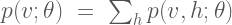
where 


Figure 1: Graphical Model of the Boltzmann machine (biases not depicted).
Given the current state of the visible and hidden units, the overall configuration of the model network is described by a connectivity function 

The parameter matrix 


The Boltzmann machine has been used for years in field of statistical mechanics to model physical systems based on the principle of energy minimization. In the statistical mechanics, the connectivity function is often referred to the “energy function,” a term that is has also been standardized in the statistical learning literature. Note that the energy function returns a single scalar value for any configuration of the network parameters and random variable states.
Given the energy function, the Boltzmann machine models the joint probability of the visible and hidden unit states as a Boltzmann distribution:
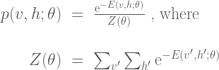
The partition function 

The common way to train the Boltzmann machine is to determine the parameters that maximize the likelihood of the observed data. To determine the parameters, we perform gradient descent on the log of the likelihood function (In order to simplify the notation in the remainder of the derivation, we do not include the explicit dependency on the parameters

The gradient calculation is as follows:
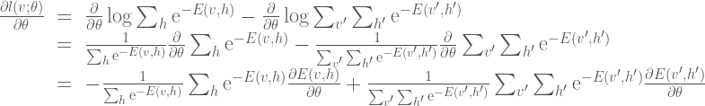
Here we can simplify the expression somewhat by noting that 


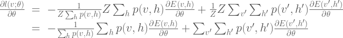
If we also note that 

Here 


Here 

MCMC: The Gibbs Sampler
In the previous post, we compared using block-wise and component-wise implementations of the Metropolis-Hastings algorithm for sampling from a multivariate probability distribution
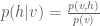
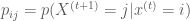
The Gibbs sampler is applicable for certain classes of problems, based on two main criterion. Given a target distribution 


Each of these expressions defines the probability of the 

The Gibbs sampler works in much the same way as the component-wise Metropolis-Hastings algorithms except that instead drawing from a proposal distribution for each dimension, then accepting or rejecting the proposed sample, we simply draw a value for that dimension according to the variable’s corresponding conditional distribution. We also accept all values that are drawn. Similar to the component-wise Metropolis-Hastings algorithm, we step through each variable sequentially, sampling it while keeping all other variables fixed. The Gibbs sampling procedure is outlined below
- set
- generate an initial state
- repeat until


set

for each dimension

draw 
To get a better understanding of the Gibbs sampler at work, let’s implement the Gibbs sampler to solve the same multivariate sampling problem addressed in the previous post.
Example: Sampling from a bivariate a Normal distribution
This example parallels the examples in the previous post where we sampled from a 2-D Normal distribution using block-wise and component-wise Metropolis-Hastings algorithms. Here, we show how to implement a Gibbs sampler to draw samples from the same target distribution. As a reminder, the target distribution
with mean
![\mu = [\mu_1,\mu_2]= [0, 0]](https://s0.wp.com/latex.php?latex=%5Cmu+%3D+%5B%5Cmu_1%2C%5Cmu_2%5D%3D+%5B0%2C+0%5D&bg=ffffff&fg=4e4e4e&s=0&c=20201002)
and covariance

In order to sample from this distribution using a Gibbs sampler, we need to have in hand the conditional distributions for variables/dimensions 


and

Where 


After some math (which which I will skip for some brevity, but see the following for some details), we find that the two conditional distributions for the target Normal distribution are:

and

which are both univariate Normal distributions, each with a mean that is dependent on the value of the most recent state of the conditioning variable, and a variance that is dependent on the target covariances between the two variables.
Using the above expressions for the conditional probabilities of variables

Gibbs sampler Markov chain and samples for bivariate Normal target distribution
Inspecting the figure above, note how at each iteration the Markov chain for the Gibbs sampler first takes a step only along the
% EXAMPLE: GIBBS SAMPLER FOR BIVARIATE NORMAL
rand('seed' ,12345);
nSamples = 5000;

mu = [0 0]; % TARGET MEAN
rho(1) = 0.8; % rho_21
rho(2) = 0.8; % rho_12

% INITIALIZE THE GIBBS SAMPLER
propSigma = 1; % PROPOSAL VARIANCE
minn = [-3 -3];
maxx = [3 3];

% INITIALIZE SAMPLES
x = zeros(nSamples,2);
x(1,1) = unifrnd(minn(1), maxx(1));
x(1,2) = unifrnd(minn(2), maxx(2));

dims = 1:2; % INDEX INTO EACH DIMENSION

% RUN GIBBS SAMPLER
t = 1;
while t < nSamples
    t = t + 1;
    T = [t-1,t];
    for iD = 1:2 % LOOP OVER DIMENSIONS
        % UPDATE SAMPLES
        nIx = dims~=iD; % *NOT* THE CURRENT DIMENSION
        % CONDITIONAL MEAN
        muCond = mu(iD) + rho(iD)*(x(T(iD),nIx)-mu(nIx));
        % CONDITIONAL VARIANCE
        varCond = sqrt(1-rho(iD)^2);
        % DRAW FROM CONDITIONAL
        x(t,iD) = normrnd(muCond,varCond);
    end
end

% DISPLAY SAMPLING DYNAMICS
figure;
h1 = scatter(x(:,1),x(:,2),'r.');

% CONDITIONAL STEPS/SAMPLES
hold on;
for t = 1:50
    plot([x(t,1),x(t+1,1)],[x(t,2),x(t,2)],'k-');
    plot([x(t+1,1),x(t+1,1)],[x(t,2),x(t+1,2)],'k-');
    h2 = plot(x(t+1,1),x(t+1,2),'ko');
end

h3 = scatter(x(1,1),x(1,2),'go','Linewidth',3);
legend([h1,h2,h3],{'Samples','1st 50 Samples','x(t=0)'},'Location','Northwest')
hold off;
xlabel('x_1');
ylabel('x_2');
axis square
Wrapping Up
The Gibbs sampler is a popular MCMC method for sampling from complex, multivariate probability distributions. However, the Gibbs sampler cannot be used for general sampling problems. For many target distributions, it may difficult or impossible to obtain a closed-form expression for all the needed conditional distributions. In other scenarios, analytic expressions may exist for all conditionals but it may be difficult to sample from any or all of the conditional distributions (in these scenarios it is common to use univariate sampling methods such as rejection sampling and (surprise!) Metropolis-type MCMC techniques to approximate samples from each conditional). Gibbs samplers are very popular for Bayesian methods where models are often devised in such a way that conditional expressions for all model variables are easily obtained and take well-known forms that can be sampled from efficiently.
Gibbs sampling, like many MCMC techniques suffer from what is often called “slow mixing.” Slow mixing occurs when the underlying Markov chain takes a long time to sufficiently explore the values of 
A Brief Introduction to Markov Chains
Markov chains are an essential component of Markov chain Monte Carlo (MCMC) techniques. Under MCMC, the Markov chain is used to sample from some target distribution. To get a better understanding of what a Markov chain is, and further, how it can be used to sample form a distribution, this post introduces and applies a few basic concepts.
A Markov chain is a stochastic process that operates sequentially (e.g. temporally), transitioning from one state to another within an allowed set of states.†

A Markov chain is defined by three elements:
- A state space
, which is a set of values that the chain is allowed to take
- A transition operator
that defines the probability of moving from state
to
.
- An initial condition distribution
which defines the probability of being in any one of the possible states at the initial iteration
.
The Markov chain starts at some initial state, which is sampled from
A Markov chain is called memoryless if the next state only depends on the current state and not on any of the states previous to the current:

(This memoryless property is formally know as the Markov property).
If the transition operator for a Markov chain does not change across transitions, the Markov chain is called time homogenous. A nice property of time homogenous Markov chains is that as the chain runs for a long time and 

We’ll see later how the stationary distribution of a Markov chain is important for sampling from probability distributions, a technique that is at the heart of Markov Chain Monte Carlo (MCMC) methods.
Finite state-space (time homogenous) Markov chain
If the state space of a Markov chain takes on a finite number of distinct values, and it is time homogenous, then the transition operator can be defined by a matrix 
This means that if the chain is currently in the 

Example: Predicting the weather with a finite state-space Markov chain
In Berkeley, CA, there are (literally) only 3 types of weather: sunny, foggy, or rainy (this is analogous to a state-space that takes on three discrete values). The weather patterns are very stable there, so a Berkeley weatherman can easily predict the weather next week based on the weather today with the following transition rules:
If it is sunny today, then
- it is highly likely that it will be sunny next week
,
- it is very unlikely that it will be raining next week
- and somewhat likely that it will foggy next week


If it is foggy today then
- it is somewhat likely that it will be sunny next week
- but slightly less likely that it will be foggy next week
,
- and fairly unlikely that it will be raining next week.
,

If it is rainy today then
- it is unlikely that it will be sunny next week
,
- it is somewhat likely that it will be foggy next week
,
- and it is fairly likely that it will be rainy next week
,
All of these transition rules can be instantiated in a single 3 x 3 transition operator matrix:

Where each row of 
% FINITE STATE-SPACE MARKOV CHAIN EXAMPLE

% TRANSITION OPERATOR
%     S  F  R
%     U  O  A
%     N  G  I
%     N  G  N
%     Y  Y  Y
P = [.8 .15 .05;  % SUNNY
     .4 .5  .1;   % FOGGY
     .1 .3  .6];  % RAINY
nWeeks = 25

% INITIAL STATE IS RAINY
X(1,:) = [0 0 1];

% RUN MARKOV CHAIN
for iB = 2:nWeeks
    X(iB,:) = X(iB-1,:)*P; % TRANSITION
end

% DISPLAY
figure; hold on
h(1) = plot(1:nWeeks,X(:,1),'r','Linewidth',2);
h(2) = plot(1:nWeeks,X(:,2),'k','Linewidth',2);
h(3) = plot(1:nWeeks,X(:,3),'b','Linewidth',2);
h(4) = plot([15 15],[0 1],'g--','Linewidth',2);
hold off
legend(h, {'Sunny','Foggy','Rainy','Burn In'});
xlabel('Week')
ylabel('p(Weather)')
xlim([1,nWeeks]);
ylim([0 1]);

% PREDICTIONS
fprintf('\np(weather) in 1 week -->'), disp(X(2,:))
fprintf('\np(weather) in 2 weeks -->'), disp(X(3,:))
fprintf('\np(weather) in 6 months -->'), disp(X(25,:))

Finite state-space Markov chain for predicting the weather
Here we see that at week 1 the probability of sunny weather is 0.1. The next week, the probability of sunny weather is 0.26, and in 6 months, there is a 60% chance that it will be sunny. Also note that after approximately 15 weeks the Markov chain has reached the equilibrium/stationary distribution and, chances are, the weather will be sunny. This 15-week period is what is known as the burn in period for the Markov chain, and is the number of transitions it takes the chain to move from the initial conditions to the stationary distribution.
A cool thing about finite state-space time-homogeneous Markov chain is that it is not necessary to run the chain sequentially through all iterations in order to predict a state in the future. Instead we can predict by first raising the transition operator to the 
![\pi^{(0)} = [0,0,1]](https://s0.wp.com/latex.php?latex=%5Cpi%5E%7B%280%29%7D+%3D+%5B0%2C0%2C1%5D&bg=ffffff&fg=4e4e4e&s=-1&c=20201002)
![p(x^{(week2)}) = \pi^{(0)}P^2 = [0.26, 0.345, 0.395]](https://s0.wp.com/latex.php?latex=p%28x%5E%7B%28week2%29%7D%29+%3D+%5Cpi%5E%7B%280%29%7DP%5E2+%3D+%5B0.26%2C+0.345%2C+0.395%5D&bg=ffffff&fg=4e4e4e&s=0&c=20201002)
and in six months:
![p(x^{(week24)}) = \pi^{(0)}P^{24} = [0.596, 0.263, 0.140]](https://s0.wp.com/latex.php?latex=p%28x%5E%7B%28week24%29%7D%29+%3D+%5Cpi%5E%7B%280%29%7DP%5E%7B24%7D+%3D+%5B0.596%2C+0.263%2C+0.140%5D&bg=ffffff&fg=4e4e4e&s=0&c=20201002)
These are the same results we get by running the Markov chain sequentially through each number of transitions. Therefore we can calculate an approximation to the stationary distribution from
Continuous state-space Markov chains
A Markov chain can also have a continuous state space that exists in the real numbers 
Example: Sampling from a continuous distribution using continuous state-space Markov chains
We can use the stationary distribution of a continuous state-space Markov chain in order to sample from a continuous probability distribution: we run a Markov chain for a sufficient amount of time so that it has reached its stationary distribution, then keep the states that the chain visits as samples from that stationary distribution.
In the following example we define a continuous state-space Markov chain. The transition operator is a Normal distribution with unit variance and a mean that is half the distance between zero and the previous state, and the distribution over initial conditions is a Normal distribution with zero mean and unit variance.
To ensure that the chain has moved sufficiently far from the initial conditions and that we are sampling from the chain’s stationary distribution, we will choose to throw away the first 50 burn in states of the chain. We can also run multiple chains simultaneously in order to sample the stationary distribution more densely. Here we choose to run 5 chains simultaneously.
% EXAMPLE OF CONTINUOUS STATE-SPACE MARKOV CHAIN

% INITIALIZE
randn('seed',12345)
nBurnin = 50; % # BURNIN
nChains = 5;  % # MARKOV CHAINS

% DEFINE TRANSITION OPERATOR
P = inline('normrnd(.5*x,1,1,nChains)','x','nChains');
nTransitions = 1000;
x = zeros(nTransitions,nChains);
x(1,:) = randn(1,nChains);

% RUN THE CHAINS
for iT = 2:nTransitions
    x(iT,:) = P(x(iT-1),nChains);
end

% DISPLAY BURNIN
figure
subplot(221); plot(x(1:100,:)); hold on;
minn = min(x(:));
maxx = max(x(:));
l = line([nBurnin nBurnin],[minn maxx],'color','k','Linewidth',2);
ylim([minn maxx])
legend(l,'~Burn-in','Location','SouthEast')
title('First 100 Samples'); hold off

% DISPLAY ENTIRE MARKOV CHAIN
subplot(223); plot(x);hold on;
l = line([nBurnin nBurnin],[minn maxx],'color','k','Linewidth',2);
legend(l,'~Burn-in','Location','SouthEast')
title('Entire Chain');

% DISPLAY SAMPLES FROM STATIONARY DISTRIBUTION
samples = x(nBurnin+1:end,:);
subplot(122);
[counts,bins] = hist(samples(:),100); colormap hot
b = bar(bins,counts);
legend(b,sprintf('Markov Chain\nSamples'));
title(['\mu=',num2str(mean(samples(:))),' \sigma=',num2str(var(samples(:)))])

Sampling from the stationary distribution of a continuous state-space Markov chain
In the upper left panel of the code output we see a close up of the first 100 of the 1000 transitions made by the 5 simultaneous Markov chains; the burn in cutoff is marked by the black line. In the lower left panel we see the entire sequence of transitions for the Markov chains. In the right panel, we can tell from the sampled states that the stationary distribution for this chain is a Normal distribution, with mean equal to zero, and a variance equal to 1.3.
Wrapping Up
In the previous example we were able to deduce the stationary distribution of the Markov chain by looking at the samples generated from the chain after the burn in period. However, in order to use Markov chains to sample from a specific target distribution, we have to design the transition operator such that the resulting chain reaches a stationary distribution that matches the target distribution. This is where MCMC methods like the Metropolis sampler, the Metropolis-Hastings sampler, and the Gibbs sampler come to rescue. We will discuss each of these Markov-chain-based sampling methods separately in later posts.
Rejection Sampling
Suppose that we want to sample from a distribution 

Envelope distribution and rejection criterion
In order to be able to reject samples from 


where 
rand('seed',12345);
x = -10:.1:10;
% CREATE A "COMPLEX DISTRIBUTION" f(x) AS A MIXTURE OF TWO NORMAL
% DISTRIBUTIONS
f = inline('normpdf(x,3,2) + normpdf(x,-5,1)','x');
t = plot(x,f(x),'b','linewidth',2); hold on;

% PROPOSAL IS A CENTERED NORMAL DISTRIBUTION
q = inline('normpdf(x,0,4)','x');

% DETERMINE SCALING CONSTANT
c = max(f(x)./q(x))

%PLOT SCALED PROPOSAL/ENVELOP DISTRIBUTION
p = plot(x,c*q(x),'k--');

% DRAW A SAMPLE FROM q(x);
qx = normrnd(0,4);
fx = f(qx);

% PLOT THE RATIO OF f(q(x)) to cq(x)
a = plot([qx,qx],[0 fx],'g','Linewidth',2);
r = plot([qx,qx],[fx,c*q(qx)],'r','Linewidth',2);
legend([t,p,a,r],{'Target','Proposal','Accept','Reject'});
xlabel('x');

Rejection Sampling with a Normal proposal distribution
Here a zero-mean Normal distribution is used as the proposal distribution. This distribution is scaled by a factor 

Rejection sampling of a random discrete distribution
This next example shows how rejection sampling can be used to sample from any arbitrary distribution, continuous or not, and with or without an analytic probability density function.

Random Discrete Target Distribution and Proposal that Bounds It.
The figure above shows a random discrete probability density function 

Rejection Samples For Discrete Distribution on interval [1 15]
rand('seed',12345)
randn('seed',12345)

fLength = 15;
% CREATE A RANDOM DISTRIBUTION ON THE INTERVAL [1 fLength]
f = rand(1,fLength); f = f/sum(f);

figure; h = plot(f,'r','Linewidth',2);
hold on;
l = plot([1 fLength],[max(f) max(f)],'k','Linewidth',2);

legend([h,l],{'f(x)','q(x)'},'Location','Southwest');
xlim([0 fLength + 1])
xlabel('x');
ylabel('p(x)');
title('Target (f(x)) and Proposal (q(x)) Distributions');

% OUR PROPOSAL IS THE DISCRETE UNIFORM ON THE INTERVAL [1 fLength]
% SO OUR CONSTANT IS
c = max(f/(1/fLength));

nSamples = 10000;
i = 1;
while i < nSamples
   proposal = unidrnd(fLength);
   q = c*1/fLength; % ENVELOPE DISTRIBUTION
   if rand < f(proposal)/q
      samps(i) = proposal;
      i = i + 1;
   end
end

% DISPLAY THE SAMPLES AND COMPARE TO THE TARGET DISTRIBUTION
bins = 1:fLength;
counts = histc(samps,bins);
figure
b = bar(1:fLength,counts/sum(counts),'FaceColor',[.8 .8 .8])
hold on;
h = plot(f,'r','Linewidth',2)
legend([h,b],{'f(x)','samples'});
xlabel('x'); ylabel('p(x)');
xlim([0 fLength + 1]);
Rejection sampling from the unit circle to estimate 
Though the ratio-based acceptance-rejection criterion introduced above is a common choice for drawing samples from complex distributions, it is not the only criterion we could use. For instance we could use a different set of criteria to generate some geometrically-bounded distribution. If we wanted to generate points uniformly within the unit circle (i.e. a circle centered at 


Unit Circle Inscribed in Square
: Because a square that inscribes the unit circle has area:
and the unit circle has the area:

We can use the ratio of their areas to approximate

The figure below shows the rejection sampling process and the resulting estimate of

Rejection Criterion
The MATLAB code used to generate the example figures is below:
% DISPLAY A CIRCLE INSCRIBED IN A SQUARE

figure;
a = 0:.01:2*pi;
x = cos(a); y = sin(a);
hold on
plot(x,y,'k','Linewidth',2)

t = text(0.5, 0.05,'r');
l = line([0 1],[0 0],'Linewidth',2);
axis equal
box on
xlim([-1 1])
ylim([-1 1])
title('Unit Circle Inscribed in a Square')

pause;
rand('seed',12345)
randn('seed',12345)
delete(l); delete(t);

% DRAW SAMPLES FROM PROPOSAL DISTRIBUTION
samples = 2*rand(2,100000) - 1;

% REJECTION
reject = sum(samples.^2) > 1;

% DISPLAY REJECTION CRITERION
scatter(samples(1,~reject),samples(2,~reject),'b.')
scatter(samples(1,reject),samples(2,reject),'rx')
hold off
xlim([-1 1])
ylim([-1 1])

piHat = mean(sum(samples.*samples)<1)*4;

title(['Estimate of \pi = ',num2str(piHat)]);
Wrapping Up
Rejection sampling is a simple way to generate samples from complex distributions. However, Rejection sampling also has a number of weaknesses:
- Finding a proposal distribution that can cover the support of the target distribution is a non-trivial task.
- Additionally, as the dimensionality of the target distribution increases, the proportion of points that are rejected also increases. This curse of dimensionality makes rejection sampling an inefficient technique for sampling multi-dimensional distributions, as the majority of the points proposed are not accepted as valid samples.
- Some of these problems are solved by changing the form of the proposal distribution to “hug” the target distribution as we gain knowledge of the target from observing accepted samples. Such a process is called Adaptive Rejection Sampling, which will be covered in another post.
Inverse Transform Sampling
There are a number of sampling methods used in machine learning, each of which has various strengths and/or weaknesses depending on the nature of the sampling task at hand. One simple method for generating samples from distributions with closed-form descriptions is Inverse Transform (IT) Sampling.
The idea behind IT Sampling is that the probability mass for a random variable 


rand('seed',12345)

% DEGREES OF FREEDOM
dF = 10;
x = -3:.1:3;
Cx = cdf('t',x,dF)
z = rand;

% COMPARE VALUES OF
zIdx = min(find(Cx>z));

% DRAW SAMPLE
sample = x(zIdx);

% DISPLAY
figure; hold on
plot(x,Cx,'k','Linewidth',2);
plot([x(1),x(zIdx)],[Cx(zIdx),Cx(zIdx)],'r','LineWidth',2);
plot([x(zIdx),x(zIdx)],[Cx(zIdx),0],'b','LineWidth',2);
plot(x(zIdx),z,'ko','LineWidth',2);
text(x(1)+.1,z + .05,'z','Color','r')
text(x(zIdx)+.05,.05,'x_{sampled}','Color','b')
ylabel('C(x)')
xlabel('x')
hold off
IT Sampling from student’s-t(10)
However, the scheme used to create to plot above is inefficient in that one must compare current values of 
- Derive
(or a good approximation) from
- for

- – draw
from
- –
- – end for
The IT sampling process is demonstrated in the next chunk of code to sample from the Beta distribution, a distribution for which
rand('seed',12345)
nSamples = 1000;

% BETA PARAMETERS
alpha = 2; beta = 10;

% DRAW PROPOSAL SAMPLES
z = rand(1,nSamples);

% EVALUATE PROPOSAL SAMPLES AT INVERSE CDF
samples = icdf('beta',z,alpha,beta);
bins = linspace(0,1,50);
counts = histc(samples,bins);
probSampled = counts/sum(counts)
probTheory = betapdf(bins,alpha,beta);

% DISPLAY
b = bar(bins,probSampled,'FaceColor',[.9 .9 .9]);
hold on;
t = plot(bins,probTheory/sum(probTheory),'r','LineWidth',2);
xlim([0 1])
xlabel('x')
ylabel('p(x)')
legend([t,b],{'Theory','IT Samples'})
hold off
Inverse Transform Sampling of Beta(2,10)
Wrapping Up
The IT sampling method is generally only used for univariate distributions where
