Blog Archives

Derivation: Maximum Likelihood for Boltzmann Machines

In this post I will review the gradient descent algorithm that is commonly used to train the general class of models known as Boltzmann machines. Though the primary goal of the post is to supplement another post on restricted Boltzmann machines, I hope that those readers who are curious about how Boltzmann machines are trained, but have found it difficult to track down a complete or straight-forward derivation of the maximum likelihood learning algorithm for these models (as I have), will also find the post informative.

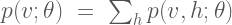
First, a little background: Boltzmann machines are stochastic neural networks that can be thought of as the probabilistic extension of the Hopfield network. The goal of the Boltzmann machine is to model a set of observed data in terms of a set of visible random variables $v$ and a set of latent/unobserved random variables $h$ . Due to the relationship between Boltzmann machines and neural networks, the random variables are often are often referred to as “units.” The role of the visible units is to approximate the true distribution of the data, while the role of the latent variables it to extend the expressiveness of the model by capturing underlying features in the observed data. The latent variables are often referred to as hidden units, as they do not result directly from the observed data and are generally marginalized over to obtain the likelihood of the observed data, i.e.

$\Large{\begin{array}{rcl} p(v;\theta) &=& \sum_h p(v,h; \theta) \end{array}}$ ,

where $p(v,h; \theta)$ is the joint probability distribution over the visible and hidden units based on the current model parameters $\theta$ . The general Boltzmann machine defines $p(v,h; \theta)$ through a set of weighted, symmetric connections between all visible and hidden units (but no connections from any unit to itself). The graphical model for the general Boltzmann machine is shown in Figure 1.

Graphical Model of the Boltzmann machine model (biases not depicted).

Figure 1: Graphical Model of the Boltzmann machine (biases not depicted).

Given the current state of the visible and hidden units, the overall configuration of the model network is described by a connectivity function $E(v,h;\theta)$ , parameterized by $\theta = {W, A, B, a, b}$ :

$\Large{\begin{array}{rcl} E(v,h; \theta) &=& v^T W h + h^T A h + v^T B v + h^T a + v^T b \end{array}}.$

The parameter matrix $W$ defines the connection strength between the visible and hidden units. The parameters $A$ and $B$ define the connection strength amongst hidden units and visible units, respectively. The model also includes a set of biases $a$ and $b$ that capture offsets for each of the hidden and visible units.

The Boltzmann machine has been used for years in field of statistical mechanics to model physical systems based on the principle of energy minimization. In the statistical mechanics, the connectivity function is often referred to the “energy function,” a term that is has also been standardized in the statistical learning literature. Note that the energy function returns a single scalar value for any configuration of the network parameters and random variable states.

Given the energy function, the Boltzmann machine models the joint probability of the visible and hidden unit states as a Boltzmann distribution:

$\Large{\begin{array}{rcl} p(v,h; \theta) &=& \frac{\mathrm{e}^{-E(v,h; \theta)}}{Z(\theta)} \text{ , where} \\ \\ Z(\theta) &=& \sum_{v'} \sum_{h'} \mathrm{e}^{-E(v',h'; \theta)}\end{array}}$

The partition function $Z(\theta)$ is a normalizing constant that is calculated by summing over all possible states of the network $(v', h') \in (V',H')$ . Here we assume that all random variables take on discrete values, but the analogous derivation holds for continuous or mixed variable types by replacing the sums with integrals accordingly.

The common way to train the Boltzmann machine is to determine the parameters that maximize the likelihood of the observed data. To determine the parameters, we perform gradient descent on the log of the likelihood function (In order to simplify the notation in the remainder of the derivation, we do not include the explicit dependency on the parameters $\theta$ . To further simplify things, let’s also assume that we calculate the gradient of the likelihood based on a single observation.):

$\Large{ \begin{array}{rcl} l(v; \theta) &=& \log p(v) \\ &=& \log \sum_h p(v,h) \\ &=& \log \frac{\sum_h \mathrm{e}^{-E(v,h)}}{Z} \\ &=& \log \sum_h \mathrm{e}^{-E(v,h)} - \log Z \\ &=& \log \sum_h \mathrm{e}^{-E(v,h)} - \sum_{v'} \sum_{h'} \mathrm{e}^{-E(v',h')} \end{array}}$

The gradient calculation is as follows:

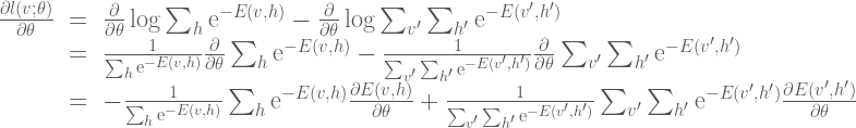
$\Large{ \begin{array}{rcl} \frac{\partial l(v;\theta)}{\partial \theta} &=& \frac{\partial}{\partial \theta}\log \sum_h \mathrm{e}^{-E(v,h)} - \frac{\partial}{\partial \theta} \log \sum_{v'}\sum_{h'}\mathrm{e}^{-E(v',h')} \\ &=& \frac{1}{\sum_h \mathrm{e}^{-E(v,h)}} \frac{\partial}{\partial \theta} \sum_h \mathrm{e}^{-E(v,h)} - \frac{1}{\sum_{v'}\sum_{h'}\mathrm{e}^{-E(v',h')}} \frac{\partial}{\partial \theta} \sum_{v'}\sum_{h'}\mathrm{e}^{-E(v',h')} \\ &=& - \frac{1}{\sum_h \mathrm{e}^{-E(v,h)}} \sum_h \mathrm{e}^{-E(v,h)}\frac{\partial E(v,h)}{\partial \theta} + \frac{1}{\sum_{v'}\sum_{h'}\mathrm{e}^{-E(v',h')}} \sum_{v'}\sum_{h'}\mathrm{e}^{-E(v',h')}\frac{\partial E(v',h')}{\partial \theta} \end{array}}$

Here we can simplify the expression somewhat by noting that $\mathrm{e}^{-E(v,h)} = Z p(v,h)$ , that $Z = \sum_{v'}\sum_{h'}\mathrm{e}^{-E(v',h')}$ , and also that $Z$ is a constant:

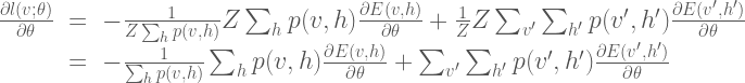
$\Large{ \begin{array}{rcl} \frac{\partial l(v;\theta)}{\partial \theta} &=& - \frac{1}{Z\sum_h p(v,h)} Z \sum_h p(v,h) \frac{\partial E(v,h)}{\partial \theta} + \frac{1}{Z} Z \sum_{v'}\sum_{h'}p(v',h')\frac{\partial E(v',h')}{\partial \theta} \\ &=& - \frac{1}{\sum_h p(v,h)} \sum_h p(v,h) \frac{\partial E(v,h)}{\partial \theta} + \sum_{v'}\sum_{h'}p(v',h')\frac{\partial E(v',h')}{\partial \theta} \\ \end{array}}$

If we also note that $\sum_h p(v,h)= p(v)$ , and use the definition of conditional probability 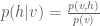$p(h|v) = \frac{p(v,h)}{p(v)}$ , we can further simplify the expression for the gradient:

$\Large{ \begin{array}{rcl} \frac{\partial l(v;\theta)}{\partial \theta} &=& - \frac{1}{p(v)} \sum_h p(v,h) \frac{\partial E(v,h)}{\partial \theta} + \sum_{v'}\sum_{h'}p(v',h')\frac{\partial E(v',h')}{\partial \theta} \\ &=& -\sum_h \frac{p(v,h)}{p(v)} \frac{\partial E(v,h)}{\partial \theta} + \sum_{v'}\sum_{h'}p(v',h')\frac{\partial E(v',h')}{\partial \theta} \\ &=& -\sum_h p(h | v) \frac{\partial E(v,h)}{\partial \theta} + \sum_{v'}\sum_{h'}p(v',h')\frac{\partial E(v',h')}{\partial \theta} \\ &=& -\mathbb{E}_{p(h | v)} \frac{\partial E(v,h)}{\partial \theta} + \mathbb{E}_{p(v',h')}\frac{\partial E(v',h')}{\partial \theta}. \\ \end{array}}$

Here $\mathbb{E}_{p(*)}$ is the expected value under the distribution $p(*)$ . Thus the gradient of the likelihood function is composed of two parts. The first part is expected gradient of the energy function with respect to the conditional distribution $p(h|v)$ . The second part is expected gradient of the energy function with respect to the joint distribution over all variable states. However, calculating these expectations is generally infeasible for any realistically-sized model, as it involves summing over a huge number of possible states/configurations. The general approach for solving this problem is to use Markov Chain Monte Carlo (MCMC) to approximate these sums:

$\Large{\begin{array}{rcl} \frac{\partial l(v;\theta)}{\partial \theta} &\approx& -\left \langle \frac{\partial E(v,h)}{\partial \theta} \right \rangle_{p(h_{\text{data}}|v_{\text{data}})} + \left \langle \frac{\partial E(v,h)}{\partial \theta} \right \rangle_{p(h_{\text{model}}|v_{\text{model}})} \\ \end{array}}.$

Here $\langle \rangle_{p(*)}$ is the sample average of samples drawn according to the process $p(*)$ . The first term is calculated by taking the average value of the energy function gradient when the visible and hidden units are being driven by observed data samples. In practice, this first term is generally straightforward to calculate. Calculating the second term is generally more complicated and involves running a set of Markov chains until they reach the current model’s equilibrium distribution (i.e. via Gibbs sampling, Metropolis-Hastings, or the like), then taking the average energy function gradient based on those samples. See this post on MCMC methods for details. It turns out that there is a subclass of Boltzmann machines that, due to a restricted connectivity/energy function (specifically, the parameters $(A, B)=0$ ), allow for efficient MCMC by way of blocked Gibbs sampling. These models, known as restricted Boltzman machines have become an important component for unsupervised pretraining in the field of deep learning and will be the focus of a related post.