Derivation: Maximum Likelihood for Boltzmann Machines

In this post I will review the gradient descent algorithm that is commonly used to train the general class of models known as Boltzmann machines. Though the primary goal of the post is to supplement another post on restricted Boltzmann machines, I hope that those readers who are curious about how Boltzmann machines are trained, but have found it difficult to track down a complete or straight-forward derivation of the maximum likelihood learning algorithm for these models (as I have), will also find the post informative.

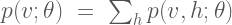
First, a little background: Boltzmann machines are stochastic neural networks that can be thought of as the probabilistic extension of the Hopfield network. The goal of the Boltzmann machine is to model a set of observed data in terms of a set of visible random variables  and a set of latent/unobserved random variables . Due to the relationship between Boltzmann machines and neural networks, the random variables are often are often referred to as “units.” The role of the visible units is to approximate the true distribution of the data, while the role of the latent variables it to extend the expressiveness of the model by capturing underlying features in the observed data. The latent variables are often referred to as hidden units, as they do not result directly from the observed data and are generally marginalized over to obtain the likelihood of the observed data,  i.e.

,

 

where is the joint probability distribution over the visible and hidden units based on the current model parameters . The general Boltzmann machine defines through a set of weighted,  symmetric connections between all visible and hidden units (but no connections from any unit to itself). The graphical model for the general Boltzmann machine is shown in Figure 1.

Figure 1: Graphical Model of the Boltzmann machine (biases not depicted).

Given the current state of the visible and hidden units, the overall configuration of the model network is described by a connectivity function , parameterized by :

The parameter matrix defines the connection strength between the visible and hidden units. The parameters and define the connection strength amongst hidden units and visible units, respectively. The model also includes a set of  biases and that capture offsets for each of the hidden and visible units.

The Boltzmann machine has been used for years in field of statistical mechanics to model physical systems based on the principle of energy minimization. In the statistical mechanics, the connectivity function is often referred to the “energy function,” a term that is has also been standardized in the statistical learning literature. Note that the energy function returns a single scalar value for any configuration of the network parameters and random variable states.

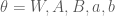
Given the energy function, the Boltzmann machine models the joint probability of the visible and hidden unit states as a Boltzmann distribution:

The partition function is a normalizing constant that is calculated by summing over all possible states of the network . Here we assume that all random variables take on discrete values, but the analogous derivation holds for continuous or mixed variable types by replacing the sums with integrals accordingly.

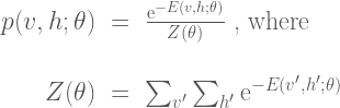
The common way to train the Boltzmann machine is to determine the parameters that maximize the likelihood of the observed data. To determine the parameters, we perform gradient descent on the log of the likelihood function (In order to simplify the notation in the remainder of the derivation, we do not include the explicit dependency on the parameters . To further simplify things, let’s also assume that we calculate the gradient of the likelihood based on a single observation.):

The gradient calculation is as follows:

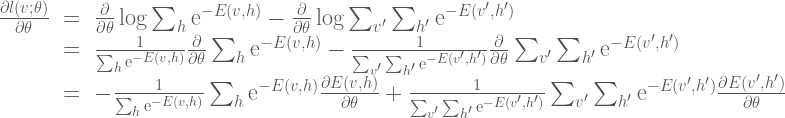
Here we can simplify the expression somewhat by noting that , that , and also that is a constant:

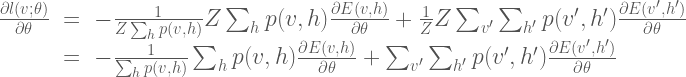
If we also note that , and use the definition of conditional probability , we can further simplify the expression for the gradient:

Here is the expected value under the distribution . Thus the gradient of the likelihood function is composed of two parts. The first part is expected gradient of the energy function with respect to the conditional distribution . The second part is expected gradient of the energy function with respect to the joint distribution over all variable states. However, calculating these expectations is generally infeasible for any realistically-sized model, as it involves summing over a huge number of possible states/configurations. The general approach for solving this problem is to use Markov Chain Monte Carlo (MCMC) to approximate these sums:

Here is the sample average of samples drawn according to the process . The first term is calculated by taking the average value of the energy function gradient when the visible and hidden units are being driven by observed data samples. In practice, this first term is generally straightforward to calculate. Calculating the second term is generally more complicated and involves running a set of Markov chains until they reach the current model’s equilibrium distribution (i.e. via Gibbs sampling, Metropolis-Hastings, or the like), then taking the average energy function gradient based on those samples. See this post on MCMC methods for details. It turns out that there is a subclass of Boltzmann machines that, due to a restricted connectivity/energy function (specifically, the parameters ), allow for efficient MCMC by way of blocked Gibbs sampling. These models, known as restricted Boltzman machines have become an important component for unsupervised pretraining in the field of deep learning and will be the focus of a related post.

A Gentle Introduction to Artificial Neural Networks

Introduction

Though many phenomena in the world can be adequately modeled using linear regression or classification, most interesting phenomena are generally nonlinear in nature. In order to deal with nonlinear phenomena, there have been a diversity of nonlinear models developed. For example parametric models assume that data follow some parameteric class of nonlinear function (e.g. polynomial, power, or exponential), then fine-tune the shape of the parametric function to fit observed data. However this approach is only helpful if data are fit nicely by the available catalog of parametric functions. Another approach, kernel-based methods, transforms data non-linearly into an abstract space that measures distances between observations, then predicts new values or classes based on these distances. However, kernel methods generally involve constructing a kernel matrix that depends on the number of training observations and can thus be prohibitive for large data sets. Another class of models, the ones that are the focus of this post, are artificial neural networks (ANNs). ANNs are nonlinear models motivated by the physiological architecture of the nervous system. They involve a cascade of simple nonlinear computations that when aggregated can implement robust and complex nonlinear functions. In fact, depending on how they are constructed, ANNs can approximate any nonlinear function, making them a quite powerful class of models (note that this property is not reserved for ANNs; kernel methods are also considered “universal approximators”; however, it turns out that neural networks with multiple layers are more efficient at approximating arbitrary functions than other methods. I refer the interested reader to more in-depth discussion on the topic.).

In recent years ANNs that use multiple stages of nonlinear computation (aka “deep learning”)  have been able obtain outstanding performance on an array of complex tasks ranging from visual object recognition to natural language processing. I find ANNs super interesting due to their computational power and their intersection with computational neuroscience.  However, I’ve found that most of the available tutorials on ANNs are either dense with formal details and contain little information about implementation or any examples, while others skip a lot of the mathematical detail and provide implementations that seem to come from thin air.  This post aims at giving a more complete overview of ANNs, including (varying degrees of) the math behind ANNs, how ANNs are implemented in code, and finally some toy examples that point out the strengths and weaknesses of ANNs.

Single-layer Neural Networks

The simplest ANN (Figure 1) takes a set of observed inputs , multiplies each of them by their own associated weight , and sums the weighted values to form a pre-activation .Oftentimes there is also a bias that is tied to an input that is always +1 included in the preactivation calculation. The network then transforms the pre-activation using a nonlinear activation function to output a final activation .

Figure 1: Diagram of a single-layered artificial neural network.

There are many options available for the form of the activation function , and the choice generally depends on the task we would like the network to perform. For instance, if the activation function is the identity function:

,

which outputs continuous values , then the network implements a linear model akin to used in standard linear regression. Another choice for the activation function is the logistic sigmoid:

,

which outputs values . When the network outputs use the logistic sigmoid activation function, the network implements linear binary classification. Binary classification can also be implemented using the hyperbolic tangent function,  , which outputs values (note that the classes must also be coded as either -1 or 1 when using . Single-layered neural networks used for classification are often referred to as “perceptrons,” a name given to them when they were first developed in the late 1950s.

Figure 2: Common activation functions functions used in artificial neural, along with their derivatives

To get a better idea of what these activation function do, their outputs for a given range of input values are plotted in the left of Figure 2. We see that the logistic and tanh activation functions (blue and green) have the quintessential sigmoidal “s” shape that saturates for inputs of large magnitude. This behavior makes them useful for categorization. The identity / linear activation (red), however forms a linear mapping between the input to the activation function, which makes it useful for predicting continuous values.

A key property of these activation functions is that they are all smooth and differentiable. We’ll see later in this post why differentiability is important for training neural networks. The derivatives for each of these common activation functions are given by (for mathematical details on calculating these derivatives,  see this post):

Each of the derivatives are plotted in the right of Figure 2. What is interesting about these derivatives is that they are either a constant (i.e. 1), or are can be defined in terms of the original function. This makes them extremely convenient for efficiently training neural networks, as we can implement the gradient using simple manipulations of the feed-forward states of the network.

Code Block 1: Defines standard activation functions and generates Figure 2:

% DEFINE A FEW COMMON ACTIVATION FUNCTIONS
gLinear = inline('z','z');
gSigmoid = inline('1./(1+exp(-z))','z');
gTanh = inline('tanh(z)','z');

% ...DEFINE THEIR DERIVATIVES
gPrimeLinear = inline('ones(size(z))','z');
gPrimeSigmoid = inline('1./(1+exp(-z)).*(1-1./(1+exp(-z)))','z');
gPrimeTanh = inline('1-tanh(z).^2','z');

% VISUALIZE EACH g(z)
z = linspace(-4,4,100);
figure
set(gcf,'Position',[100,100,960,420])
subplot(121);  hold on;
h(1) = plot(z,gLinear(z),'r','Linewidth',2);
h(2) = plot(z,gSigmoid(z),'b','Linewidth',2);
h(3) = plot(z,gTanh(z),'g','Linewidth',2);
set(gca,'fontsize',16)
xlabel('z')
legend(h,{'g_{linear}(z)','g_{logistic}(z)','g_{tanh}(z)'},'Location','Southeast')
title('Some Common Activation Functions')
hold off, axis square, grid
ylim([-1.1 1.1])

% VISUALIZE EACH g'(z)
subplot(122); hold on
h(1) = plot(z,gPrimeLinear(z),'r','Linewidth',2);
h(2) = plot(z,gPrimeSigmoid(z),'b','Linewidth',2);
h(3) = plot(z,gPrimeTanh(z),'g','Linewidth',2);
set(gca,'fontsize',16)
xlabel('z')
legend(h,{'g''_{linear}(z)','g''_{logistic}(z)','g''_{tanh}(z)'},'Location','South')
title('Activation Function Derivatives')
hold off, axis square, grid
ylim([-.5 1.1])

 

Multi-layer Neural Networks

As was mentioned above, single-layered networks implement linear models, which doesn’t really help us if we want to model nonlinear phenomena. However, by considering the single layer network  diagrammed in Figure 1 to be a basic building block, we can construct more complicated networks, ones that perform powerful, nonlinear computations. Figure 3 demonstrates this concept. Instead of a single layer of weights between inputs and output, we introduce a set of  single-layer networks between the two. This set of intermediate networks is often referred to as a “hidden” layer, as it doesn’t directly observe input or directly compute the output. By using a hidden layer, we form a mult-layered ANN. Though there are many different conventions for declaring the actual number of layers in a multi-layer network, for this discussion we will use the convention of the number of distinct sets of trainable weights as the number of layers. For example, the network in Figure 3 would be considered a 2-layer ANN because it has two layers of weights: those connecting the inputs to the hidden layer (), and those connecting the output of the hidden layer to the output layer().

Figure 3: Diagram of a multi-layer ANN. Each node in the network can be considered a single-layered ANN (for simplicity, biases are not visualized in graphical model)

Multi-layer neural networks form compositional functions that map the inputs nonlinearly to outputs. If we associate index i with the input layer, index j with the hidden layer, and index k with the output layer, then an output unit in the network diagrammed in Figure 3 computes an output value given and input via the following compositional function:

.

Here is the  is the pre-activation values for units for layer , is the activation function for units  in that layer (assuming they are the same), and is the output activation for units in that layer. The weight links the outputs of units feeding into layer to the activation function of units for that layer. The term is the bias for units in layer .

As with the single-layered ANN, the choice of activation function for the output layer will depend on the task that we would like the network to perform (i.e. categorization or regression), and follows similar rules outlined above. However, it is generally desirable for the hidden units to have nonlinear activation functions (e.g. logistic sigmoid or tanh). This is because multiple layers of linear computations can be equally formulated as a single layer of linear computations. Thus using linear activations for the hidden layers doesn’t buy us much. However, as we’ll see shortly, using linear activations for the output unit activation function (in conjunction with nonlinear activations for the hidden units) allows the network to perform nonlinear regression.

Training neural networks & gradient descent

Training neural networks involves determining the network parameters that minimize the errors that the network makes. This first requires that we have a way of quantifying error. A standard way of quantifying error is to take the squared difference between the network output and the target value:

(Note that the squared error is not chosen arbitrarily, but has a number of theoretical benefits and considerations. For more detail, see the following post) With an error function in hand, we then aim to find the setting of parameters that minimizes this error function. This concept can be interpreted spatially by imagining a “parameter space” whose dimensions are the values of each of the model parameters, and for which the error function will form a surface of varying height depending on its value for each parameter. Model training is thus equivalent to finding point in parameter space that makes the height of the error surface small.

To get a better intuition behind this concept, let’s define a super simple neural network, one that has a single input and a single output (Figure 4, bottom left). For further simplicity, we’ll assume the network has no bias term and thus has a single parameter, . We will also assume that the output layer uses the logistic sigmoid activation function. Accordingly, the network will map some input value onto a predicted output via the following function.

Now let’s say we want this simple network to learn the identity function: given an input of 1 it should return a target value of 1. Given this target value we can now calculate the value of the error function for each setting of . Varying the value of from -10 to 10 results in the error surface displayed in the left of Figure 4.  We see that the error is small for large positive values of , while the error is large for strongly negative values of . This not surprising, given that the output activation function is the logistic sigmoid, which will map large values onto an output of 1.

Things become more interesting when we move from a single-layered network to a multi-layered network. Let’s repeat the above exercise, but include a single hidden node between the input and the output (Figure 4, bottom right). Again, we will assume no biases, and logistic sigmoid activations for both the hidden and output nodes. Thus the network will have two parameters: . Accordingly the 2-layered network will predict an output with the  following function:

Now, if we vary both and , we obtain the error surface in the right of Figure 4.

Figure 4: Error surface for a simple, single-layer neural network (left) and a 2-layer network (right). The goal is to map the input value 1 to the output value 1.

 

We see that the error function is minimized when both and are large and positive. We also see that the error surface is more complex than for the single-layered model, exhibiting a number of wide plateau regions. It turns out that the error surface gets more and more complicated as you increase the number of layers in the network and the number of units in each hidden layer. Thus, it is important to consider these phenomena when constructing neural network models.

Code Block 2: generates Figure 4 (assumes you have run Code Block 1):

% VISUALIZE ERROR SURFACE OF SIMPLE ANNS
E = {};
[w1,w2] = meshgrid(linspace(-10,10,50));
g = gSigmoid;
target = 1;
net1Output = g(w1.*target);
net2Output = g(w2.*g(w1.*target));
E{1} = (net1Output - target).^2;
E{2} = (net2Output - target).^2;
figure
for ii = 1:2
	set(gcf,'Position',[100,100,960,420])
	subplot(1,2,ii)
	surf(w1,w2,E{ii}); shading faceted;
	colormap(flipud(hot)); caxis([0,max(max(E{ii}))])
	set(gca,'fontsize',16)
	xlabel('w_{1}'), ylabel('w_{2}'), zlabel('E(w)')
	axis square;
	title(sprintf('Error Surface: %d-layer Network',ii))
	[az, el] = view;
	view([az + 180, el]);
	set(gcf,'position',[100,100,1020,440])
	drawnow
end

The examples in Figure 4 gives us a qualitative idea of how to train the parameters of an ANN, but we would like a more automatic way of doing so. Generally this problem is solved  using gradient descent: The gradient descent algorithm first calculates the derivative / gradient of the error function with respect  to each of the model parameters. This gradient information will give us the direction in parameter space that decreases the height of the error surface. We then take a step in that direction and repeat, iteratively calculating the gradient and taking steps in parameter space.

The backpropagation algorithm

It turns out that the gradient information for the ANN error surface can be calculated efficiently using a message passing algorithm known as the backpropagation algorithm. During backpropagation, input signals are forward-propagated through the network toward the outputs, and network errors are then calculated with respect to target variables and back-propagated backwards towards the inputs. The forward and backward signals are then used to determine the direction in the parameter space to move that lowers the network error.

The formal calculations behind the backpropagation algorithm can be somewhat mathematically involved and may detract from the general ideas behind the learning algorithm. For those readers who are interested in the math, I have provided the formal derivation of the backpropagation algorithm in the following post (for those of you who are not interested in the math, I would also encourage you go over the derivation and try to make connections to the source code implementations provided later in the post).

Figure 5 demonstrates the key steps of the backpropagation algorithm. The main concept underlying the algorithm is that for a given observation we want to determine the degree of “responsibility” that each network parameter has for mis-predicting a target value associated with the observation. We then change that parameter according to this responsibility so that it reduces the network error.

Figure 5: The 4 main steps of the bacdkpropagation algorithm: I Forward propagate error signals to output, II Calculate output error E, and backpropagate error signal, III Use forward signal and backward signals to calculate parameter gradients, IV update network parameters.

In order to determine the network error, we first propagate the observed input forward through the network layers. This is Step I of the backpropagation algorithm, and is demonstrated in Figure 5-I. Note that in the Figure  could be considered network output  (for a network with one hidden layer) or the output of a hidden layer that projects the remainder of the network (in the case of a network with more than one hidden layer). For this discussion, however, we assume that the index k is associated with the output layer of the network, and thus each of the network outputs is designated by . Also note that when implementing this forward-propagation step, we should keep track of the feed-forward pre-activations and activations for all layers , as these will be used for calculating backpropagated errors and error function gradients.

Step II of the algorithm is to calculate the network output error and backpropagate it toward the input. Let’s again that we are using the sum of squared differences error function:

,

where we sum over the values of all output units (one in this example). We can now define an “error signal”   at the output node that will be backpropagated toward the input. The error signal is calculated as follows:

.

Thus the error signal essentially weights the gradient of the error function by the gradient of the output activation function (notice there is a term is used in this calculation, which is why we keep it around during the forward-propagation step). We can continue backpropagating the error signal toward the input by passing through the output layer weights , summing over all output nodes, and passing the result through the gradient of the activation function at the hidden layer (Figure 5-II). Performing these operations results in the back-propagated error signal for the hidden layer, :

,

For networks that have more than one hidden layer, this error backpropagation procedure can continue for layers , etc.

Step III of the backpropagation algorithm is to calculate the gradients of the error function with respect to the model parameters at each layer using the forward signals , and the backward error signals . If one considers the model weights  at a layer as linking the forward signal to the error signal (Figure 5-III), then the gradient of the error function with respect to those weights is:

Note that this result is closely related to the concept of Hebbian learning in neuroscience. Thus the gradient of the error function with respect to the model weight at each layer can be efficiently calculated by simply keeping track of the forward-propagated activations feeding into that layer from below, and weighting those activations by the backward-propagated error signals feeding into that layer from above!

What about the bias parameters? It turns out that the same gradient rule used for the weight weights applies, except that “feed-forward activations” for biases are always +1 (see Figure 1). Thus the bias gradients for layer are simply:

The fourth and final step of the backpropagation algorithm is to update the model parameters based on the gradients calculated in Step III. Note that the gradients point in the direction in parameter space that will increase the value of the error function. Thus when updating the model parameters we should choose to go in the opposite direction. How far do we travel in that direction? That is generally determined by a user-defined step size (aka learning rate) parameter, . Thu,s given the parameter gradients and the step size, the weights and biases for a given layer are updated accordingly:

.

To train an ANN, the four steps outlined above and in Figure 5 are repeated iteratively by observing many input-target pairs and updating the parameters until either the network error reaches a tolerably low value, the parameters cease to update (convergence), or a set number of parameter updates has been achieved. Some readers may find the steps of the backpropagation somewhat ad hoc. However, keep in mind that these steps are formally coupled to the calculus of the optimization problem. Thus I again refer the curious reader to check out the derivation in order to make connections between the algorithm and the math.

Example: learning the OR & AND logical operators using a single layer neural network

Here we go over an example of training a single-layered neural network to perform a classification problem. The network is trained to learn a set of logical operators including the  AND, OR, or XOR. To train the network we first generate training data. The inputs consist of 2-dimensional coordinates that span the input values values for a 2-bit truth table:

Figure 6: Truth table values learned in classification examples

We then perturb these observations by adding Normally-distributed noise. To generate target variables, we categorize each observations by applying one of logic operators (See Figure 6) to the original (no-noisy) coordinates. We then train the network with the noisy inputs and binary categories targets using the gradient descent / backpropagation algorithm. The code implementation of the network and training procedures, as well as the resulting learning process are displayed below. (Note that in this implementation, I do not use the feed-forward activations to calculate the gradients as suggested above. This is simply to make the implementation of the learning algorithm more explicit in terms of the math. The same situation also applies to the other examples in this post).

Code Block 3: Implements and trains a single-layer neural network for classification to learn logical operators (assumes you have run Code Block 1):

%% EXAMPLE: SINGLE-LAYERED NETWORK

% DEFINE DATA AND TARGETS
data = [0 0; 0 1; 1 0; 1 1;];
classAND = and(data(:,1)>0,data(:,2)>0);
classOR = or(data(:,1)>0,data(:,2)>0);
classXOR = xor(data(:,1)>0,data(:,2)>0);

% THE TYPE OF TRUTH TABLE TO LEARN (UNCOMMENT FOR OTHERS)
classes = classOR
% classes = classAND;
% classes = classXOR;

% MAKE MULTIPLE NOISY TRAINING OBSERVATIONS
nRepats = 30;
data = repmat(data, [nRepats, 1]);
classes = repmat(classes, [nRepats, 1]);
data = data + .15*randn(size(data));

% SHUFFLE DATA
shuffleIdx = randperm(size(data,1));
data = data(shuffleIdx,:);
classes = classes(shuffleIdx);

% INITIALIZE MODEL PARAMETERS
[nObs,nInput] = size(data); % # OF INPUT DIMENSIONS
nOutput = 1;    			% # OF TARGET/OUTPUT DIMENSIONS
lRate = 3;    				% LEARNING RATE FOR PARAMETERS UPDATE
nIters = 80;  				% # OF ITERATIONS

% DECLARE ACTIVATION FUNCTIONS (AND DERIVATIVES)
g_out = gSigmoid; gPrime_out = gPrimeSigmoid;

% INITIALIZE RANDOM WEIGHTS
W_out = (rand(nInput,nOutput)-.5);
b_out = (rand(1,nOutput)-.5);

% SOME OTHER INITIALIZATIONS
% (FOR VISUALIZATION)
visRange = [-.2 1.2];
[xx,yy] = meshgrid(linspace(visRange(1), visRange(2),100));
iter = 1;
mse = zeros(1,nIters);

figure
set(gcf,'Position',[100,100,960,420])
while 1
	err = zeros(1,nObs);
	% LOOP THROUGH THE EXAMPLES
	for iO = 1:nObs

		% GET CURRENT NETWORK INPUT DATA AND TARGET
		input = data(iO,:);
		target = classes(iO);

		%% I. FORWARD PROPAGATE DATA THROUGH NETWORK
		z_out = input*W_out + b_out; % OUTPUT UNIT PRE-ACTIVATIONS
		a_out = g_out(z_out);        % OUTPUT UNIT ACTIVATIONS

		%% II. BACKPROPAGATE ERROR SIGNAL
		% CALCULATE ERROR DERIVATIVE W.R.T. OUTPUT
		delta_out = gPrime_out(z_out).*(a_out - target);

		%% III. CALCULATE GRADIENT W.R.T. PARAMETERS...
		dEdW_out = delta_out*input;
		dEdb_out = delta_out*1;

		%% IV. UPDATE NETWORK PARAMETERS
		W_out = W_out - lRate*dEdW_out';
		b_out = b_out - lRate*dEdb_out';

		% CALCULATE ERROR FUNCTION
		err(iO) = .5*(a_out-target).^2;
	end
	mse(iter) = mean(err);

	% DISPLAY LEARNING
	clf; subplot(121); hold on;
	set(gca,'fontsize',16)
	netOut = g_out(bsxfun(@plus,[xx(:),yy(:)]*W_out, b_out));
	contourf(xx,yy,reshape(netOut,100,100)); colormap(flipud(spring))
	hold on;
	gscatter(data(:,1),data(:,2),classes,[0 0 0 ; 1 1 1],[],20,'off');
	title(sprintf('Iteration %d',iter))
	xlim([visRange(1) visRange(2)]),ylim([visRange(1) visRange(2)]);
	axis square

	subplot(122);
	set(gca,'fontsize',16)
	plot(1:iter,mse(1:iter));
	xlabel('Iteration')
	ylabel('Mean Squared Error')
	axis square
	m1(iter) = getframe(gcf);

	if iter >= nIters
		break
	end
	iter = iter + 1;
end

Figure 7: Single layer neural network (perceptron) learning a noisy OR mapping.

Figure 7 displays the procedure for learning the OR mapping. The left plot displays the training data and the network output at each iteration. White dots are training points categorized “1” while black dots are categorized “0”. Yellow regions are where the network predicts values of “0”, while magenta highlights areas where the network predicts “1”. We see that the single-layer network is able to easily separate the two classes.  The right plot shows how the error function decreases with each training iteration. The smooth trajectory of the error indicates that the error surface is also fairly smooth.

Figure 8: Single layer neural network (perceptron) learning a noisy AND mapping.

Figure 8 demonstrates an analogous example, but instead learning the AND operator (by executing Code Block 3, after un-commenting line 11). Again, the  categories can be easily separated by a plane, and thus the single-layered network easily learns an accurate predictor of the data.

Going Deeper: nonlinear classification and multi-layer neural networks

Figures 7 and 8 demonstrate how a single-layered ANN can easily learn the OR and AND operators. This is because the categorization criterion for these logical operators can be represented in the input space by a single linear function (i.e. line/plane). What about more complex categorization criterion that cannot be represented by a single plane? An example of a more complex binary classification criterion is the XOR operator (Figure 6, far right column).

Below we attempt to train the single-layer network to learn the XOR operator (by executing Code Block 3, after un-commenting line 12). The single layer network is unable to learn this nonlinear mapping between the inputs and the targets. However, it turns out we can learn the XOR operator using a multi-layered neural network.

Figure 9: Single layer neural network (perceptron) attempting to learn a noisy XOR mapping. The single layer network chokes on this nonlinear problem.

Below we train a two-layer neural network on the XOR dataset. The network incorporates a hidden layer with 3 hidden units and logistic sigmoid activation functions for all units in the hidden and output layers (see Code Block 4, lines 32-33).

Code Block 4: Implements and trains a two-layer neural network for classification to learn XOR operator and more difficult “ring” problem (Figures 10 & 11; assumes you have run Code Block 1):

%% EXAMPLE: MULTI-LAYER NEURAL NETWORK FOR CLASSIFICATION
data = [0 0; 0 1; 1 0; 1 1;];
classXOR = xor(data(:,1)>0,data(:,2)>0);

% THE TYPE OF TRUTH TABLE TO LEARN
classes = classXOR;

% UNCOMMENT FOR MOR DIFFICULT DATA...
% data = [data; .5 .5; 1 .5; 0 .5; .5 0; .5 1];
% classRing = [1; 1; 1; 1; 0; 1; 1; 1; 1];
% classes = classRing;

% CREATE MANY NOISY OBSERVATIONS
nRepats = 30;
data = repmat(data, [nRepats, 1]);
classes = repmat(classes, [nRepats, 1]);
data = data + .15*randn(size(data));

% SHUFFLE OBSERVATIONS
shuffleIdx = randperm(size(data,1));
data = data(shuffleIdx,:);
classes = classes(shuffleIdx);

% INITIALIZE MODEL PARAMETERS
[nObs,nInput] = size(data);   	% # OF INPUT DIMENSIONS
nHidden = 3;    				% # OF HIDDEN UNITS

lRate = 2;    	% LEARNING RATE FOR PARAMETERS UPDATE
nIters = 300;   % # OF ITERATIONS

% DECLARE ACTIVATION FUNCTIONS (AND DERIVATIVES)
g_hid = gSigmoid; gPrime_hid = gPrimeSigmoid;
g_out = gSigmoid; gPrime_out = gPrimeSigmoid;

% INITIALIZE WEIGHTS
W_hid = (rand(nInput,nHidden)-.5);
b_hid = (rand(1,nHidden)-.5);
W_out = (rand(nHidden,nOutput)-.5);
b_out = (rand(1,nOutput)-.5);

iter = 1;
mse = zeros(1,nIters);
figure
set(gcf,'Position',[100,100,960,420])
% MAIN TRAINING ALGORITHM
while 1
	err = zeros(1,nObs);
	% LOOP THROUGH THE EXAMPLES
	for iO = 1:nObs

		% GET CURRENT NETWORK INPUT DATA AND TARGET
		input = data(iO,:);
		target = classes(iO);

		%% I. FORWARD PROPAGATE DATA THROUGH NETWORK
		z_hid = input*W_hid + b_hid; % HIDDEN UNIT PRE-ACTIVATIONS
		a_hid = g_hid(z_hid);        % HIDDEN UNIT ACTIVATIONS
		z_out = a_hid*W_out + b_out; % OUTPUT UNIT PRE-ACTIVATIONS
		a_out = g_out(z_out);        % OUTPUT UNIT ACTIVATIONS

		%% II.  BACKPROPAGATE ERROR SIGNAL
		% CALCULATE ERROR DERIVATIVE W.R.T. OUTPUT
		delta_out = gPrime_out(z_out).*(a_out - target);

		% CALCULATE ERROR CONTRIBUTIONS FOR HIDDEN NODES...
		delta_hid = gPrime_hid(z_hid)'.*(delta_out*W_out);

		%% III. CALCULATE GRADIENT W.R.T. PARAMETERS...
		dEdW_out = delta_out*a_hid;
		dEdb_out = delta_out*1;
		dEdW_hid = delta_hid*input;
		dEdb_hid = delta_hid*1;

		%% IV. UPDATE NETWORK PARAMETERS
		W_out = W_out - lRate*dEdW_out';
		b_out = b_out - lRate*dEdb_out';

		W_hid = W_hid - lRate*dEdW_hid';
		b_hid = b_hid - lRate*dEdb_hid';

		% CALCULATE ERROR FUNCTION
		err(iO) = .5*(a_out-target).^2;
	end
	mse(iter) = mean(err);

	% DISPLAY LEARNING
	clf; subplot(121); hold on;
	set(gca,'fontsize',16)

	netOut = g_out(bsxfun(@plus,g_hid(bsxfun(@plus,[xx(:),yy(:)]*W_hid, b_hid))*W_out, b_out));
	contourf(xx,yy,reshape(netOut,100,100)); colormap(flipud(spring))
	hold on;
	gscatter(data(:,1),data(:,2),classes,[0 0 0; 1 1 1],[],20,'off');
	title(sprintf('Iteration %d',iter))
	xlim([visRange(1), visRange(2)]),ylim([visRange(1), visRange(2)]);
	axis square

	subplot(122);
	set(gca,'fontsize',16)
	plot(1:iter,mse(1:iter));
	xlabel('Iteration')
	ylabel('Mean Squared Error')
	axis square
	m2(iter) = getframe(gcf);

	if iter >= nIters
		break
	end
	iter = iter + 1;
end

Figure 10: A multi-layer neural network (perceptron) attempting to learn a noisy XOR mapping. The multi-layer network easily learns this nonlinear problem.

Figure 10 displays the learning process for the 2-layer network. The formatting for Figure 10 is analogous to that for Figures 7-9. The 2-layer network is easily able to learn the XOR operator. We see that by adding a hidden layer between the input and output, the ANN is able to learn the nonlinear categorization criterion!

Figure 11 shows the results for learning a even more difficult nonlinear categorization function: points in and around are categorized as “0”, while points in a ring surrounding the “0” datapoints are categorized as a “1” (Figure 11). This example is run by executing Code Block 4 after un-commenting  lines 9-11.

Figure 11: Multilayer neural network learning a nonlinear binary classification task

Figure 11 shows the learning process. Again formatting is analogous to the formatting in Figures 8-10. The 2-layer ANN is able to learn this difficult classification criterion.

Example: Neural Networks for Regression

The previous examples demonstrated how ANNs can be used for classification by using a logistic sigmoid as the output activation function. Here we demonstrate how, by making the output activation function the linear/identity function, the same 2-layer network architecture can be used to implement nonlinear regression.

For this example we define a dataset comprised of 1D inputs, that range from . We then generate noisy targets according to the function:

where is a nonlinear data-generating function and is Normally-distributed noise. We then construct a two-layered network with tanh activation functions used in the hidden layer and linear outputs. For this example we set the number of hidden units to 3 and train the model as we did for categorization using gradient descent / backpropagation. The results of the example are displayed below.

Code Block 5: Trains two-layer network for regression problems (Figures 11 & 12; assumes you have run Code Block 1):

%% EXAMPLE: NONLINEAR REGRESSION

% DEFINE DATA-GENERATING FUNCTIONS f(x)
xMin = -5; xMax = 5;
xx = linspace(xMin, xMax, 100);
f = inline('2.5 + sin(x)','x');
% f = inline('abs(x)','x'); % UNCOMMENT FOR FIGURE 13
yy = f(xx) + randn(size(xx))*.5;

% FOR SHUFFLING OBSERVATIONS
shuffleIdx = randperm(length(xx));
data = xx;
targets = yy;

% INITIALIZE MODEL PARAMETERS
nObs = length(data); 	% # OF INPUT DIMENSIONS
nInput = 1;				% # OF INPUTS
nHidden = 3; 			% # OF HIDDEN UNITS
nOutput = 1;			% # OF TARGET/OUTPUT DIMENSIONS
lRate = .15;   			% LEARNING RATE FOR PARAMETERS UPDATE
nIters = 200;  			% # OF ITERATIONS

cols = lines(nHidden);

% DECLARE ACTIVATION FUNCTIONS (AND DERIVATIVES)
g_hid = gTanh;  		   % HIDDEN UNIT ACTIVATION
gPrime_hid = gPrimeTanh;   % GRAD OF HIDDEN UNIT ACTIVATION
g_out = gLinear; 		   % OUTPUT ACTIVATION
gPrime_out = gPrimeLinear; % GRAD. OF OUTPUT ATIVATION

% % INITIALIZE WEIGHTS
W_hid = (rand(nInput,nHidden)-.5);
b_hid = (rand(1,nHidden)-.5);
W_out = (rand(nHidden,nOutput)-.5);
b_out = (rand(1,nOutput)-.5);

% INITIALIZE SOME THINGS..
% (FOR VISUALIZATION)
mse = zeros(1,nIters);
visRange = [xMin, xMax];
figure
set(gcf,'Position',[100,100,960,420])
iter = 1;
while 1

	err = zeros(1,nObs);
	% LOOP THROUGH THE EXAMPLES
	for iO = 1:nObs

		% GET CURRENT NETWORK INPUT DATA AND TARGET
		input = data(iO);
		target = targets(iO);

		%% I. FORWARD PROPAGATE DATA THROUGH NETWORK
		z_hid = input*W_hid + b_hid; % HIDDEN UNIT PRE-ACTIVATIONS
		a_hid = g_hid(z_hid);        % HIDDEN UNIT ACTIVATIONS
		z_out = a_hid*W_out + b_out; % OUTPUT UNIT PRE-ACTIVATIONS
		a_out = g_out(z_out);        % OUTPUT UNIT ACTIVATIONS

		%% II. BACKPROPAGATE ERROR SIGNAL
		% CALCULATE ERROR DERIVATIVE W.R.T. OUTPUT
		delta_out = gPrime_out(z_out).*(a_out - target);

		%% CALCULATE ERROR CONTRIBUTIONS FOR HIDDEN NODES...
		delta_hid = gPrime_hid(z_hid)'.*(delta_out*W_out);

		%% III. CALCULATE GRADIENT W.R.T. PARAMETERS...
		dEdW_out = delta_out*a_hid;
		dEdb_out = delta_out*1;
		dEdW_hid = delta_hid*input;
		dEdb_hid = delta_hid*1;

		%% IV. UPDATE NETWORK PARAMETERS
		W_out = W_out - lRate*dEdW_out';
		b_out = b_out - lRate*dEdb_out';

		W_hid = W_hid - lRate*dEdW_hid';
		b_hid = b_hid - lRate*dEdb_hid';

		% CALCULATE ERROR FUNCTION FOR BATCH
		err(iO) = .5*(a_out-target).^2;
	end
	mse(iter) = mean(err); % UPDATE ERROR

	% DISPLAY LEARNING
	clf; subplot(121); hold on;
	set(gca,'fontsize',14)

	plot(xx,f(xx),'m','linewidth',2);
	hold on;
	scatter(xx, yy ,'m');

	% PLOT TOTAL NETWORK OUTPUT
	netOut = g_out(g_hid(bsxfun(@plus, xx'*W_hid, b_hid))*W_out + b_out);
	plot(xx, netOut, 'k','linewidth', 2)

	% PLOT EACH HIDDEN UNIT'S OUTPUT FUNCTION
	for iU = 1:nHidden
		plot(xx,g_hid(xx*W_hid(iU) + b_hid(iU)),'color',cols(iU,:),'Linewidth',2, ...
                                                                           'Linestyle','--');
	end

	% TITLE AND LEGEND
	title(sprintf('Iteration %d',iter))
	xlim([visRange(1) visRange(2)]),ylim([visRange(1) visRange(2)]);
	axis square
	legend('f(x)', 'Targets', 'Network Output','Hidden Unit Outputs','Location','Southwest')

	% PLOT ERROR
	subplot(122);
	set(gca,'fontsize',14)
	plot(1:iter,mse(1:iter));
	xlabel('Iteration')
	ylabel('Mean Squared Error')
	axis square; drawnow

	% ANNEAL LEARNING RATE
	lRate = lRate *.99;
	if iter >= nIters
		break
	end
	iter = iter + 1;
end

Figure 12: A two-layered ANN used for regression. The network approximates the function f(x) = sin(x) + 2.5

The training procedure for is visualized in the left plot of Figure 12. The data-generating function is plotted as the solid magenta line, and the noisy target values used to train the network are plotted as magenta circles. The output of the network at each training iteration is plotted in solid black while the output of each of the tanh hidden units is plotted in dashed lines. This visualization demonstrates how multiple nonlinear functions can be combined to form the complex output target function. The mean squared error at each iteration is plotted in the right plot of Figure 12. We see that the error does not follow a simple trajectory during learning, but rather undulates, demonstrating the non-convexity of the error surface.

Figure 13 visualizes the training procedure for trying to learn a different nonlinear function, namely (by running Code Block 5, after un-commenting out line 7). Again, we see how the outputs of the hidden units are combined to fit the desired data-generating function. The mean squared error again follows an erratic path during learning.

Figure 13: A two-layered ANN used for regression. The network approximates the function f(x) = abs(x)

Notice for this example that I added an extra implementation detail known as simulated annealing (line 118) that was absent in the classification examples. This technique decreases the learning rate after every iteration thus making the algorithm take smaller and smaller steps in parameter space.  This technique can be useful when the gradient updates begin oscillating between two or more locations in the parameter space. It is also helpful for influencing the algorithm to settle down into a steady state.

Wrapping up

In this post we covered the main ideas behind artificial neural networks including: single- and multi-layer ANNs, activation functions and their derivatives, a high-level description of the backpropagation algorithm, and a number of classification and regression examples. ANNs, particularly mult-layer ANNs, are a robust and powerful class of models that can be used to learn complex, nonlinear functions. However, there are a number of considerations when using neural networks including:

• How many hidden layers should one use?
• How many hidden units in each layer?
• How do these relate to overfitting and generalization?
• Are there better error functions than the squared difference?
• What should the learning rate be?
• What can we do about the complexity of error surface with deep networks?
• Should we use simulated annealing?
• What about other activation functions?

It turns out that there are no easy or definite answers to any of these questions, and there is active research focusing on each topic. This is why using ANNs is often considered as much as a “black art” as it is a quantitative technique.

One primary limitation of ANNs is that they are supervised algorithms, requiring a target value for each input observation in order to train the network. This can be prohibitive for training large networks that may require lots of training data to adequately adjust the parameters. However, there are a set of unsupervised variants of ANNs that can be used to learn an initial condition for the ANN (rather than from randomly-generated initial weights) without the need of target values. This technique of “unsupervised pretraining” has been an important component of many “deep learning” models used in AI and machine learning. In future posts, I look forward to covering two of these unsupervised neural networks: autoencoders and restricted Boltzmann machines.

 

Derivation: Derivatives for Common Neural Network Activation Functions

Introduction

When constructing Artificial Neural Network (ANN) models, one of the primary considerations is choosing activation functions for hidden and output layers that are differentiable. This is because calculating the backpropagated error signal that is used to determine ANN parameter updates requires the gradient of the activation function gradient . Three of the most commonly-used activation functions used in ANNs are the identity function, the logistic sigmoid function, and the hyperbolic tangent function. Examples of these functions and their associated gradients (derivatives in 1D) are plotted in Figure 1.

Common activation functions functions used in artificial neural, along with their derivatives

In the remainder of this post, we derive the derivatives/gradients for each of these common activation functions.

The Identity Activation Function

The simplest activation function, one that is commonly used for the output layer activation function in regression problems,  is the identity/linear activation function:

(Figure 1, red curves). This activation function simply maps the pre-activation to itself and can output values that range . Why would one want to do use an identity activation function? After all, a multi-layered network with linear activations at each layer can be equally-formulated as a single-layered linear network. It turns out that the identity activation function is surprisingly useful. For example, a multi-layer network that has nonlinear activation functions amongst the hidden units and an output layer that uses the identity activation function implements a powerful form of nonlinear regression. Specifically, the network can predict continuous target values using a linear combination of signals that arise from one or more layers of nonlinear transformations of the input.

The derivative of ,  ,  is simply 1, in the case of 1D inputs. For vector inputs of length the gradient is , a vector of ones of length .

The Logistic Sigmoid Activation Function

Another function that is often used as the output activation function for binary classification problems (i.e. outputs values that range ), is the logistic sigmoid. The logistic sigmoid has the following form:

(Figure 1, blue curves) and outputs values that range . The logistic sigmoid is motivated somewhat by biological neurons and can be interpreted as the probability of an artificial neuron “firing” given its inputs. (It turns out that the logistic sigmoid can also be derived as the maximum likelihood solution to for logistic regression in statistics). Calculating the derivative of the logistic sigmoid function makes use of the quotient rule and a clever trick that both adds and subtracts a one from the numerator:

Here we see that evaluated at is simply weighted by 1-minus-. This turns out to be a convenient form for efficiently calculating gradients used in neural networks: if one keeps in memory the feed-forward activations of the logistic function for a given layer, the gradients for that layer can be evaluated using simple multiplication and subtraction rather than performing any re-evaluating the sigmoid function, which requires extra exponentiation.

The Hyperbolic Tangent Activation Function

Though the logistic sigmoid has a nice biological interpretation, it turns out that the logistic sigmoid can cause a neural network to get “stuck” during training. This is due in part to the fact that if a strongly-negative input is provided to the logistic sigmoid, it outputs values very near zero. Since neural networks use the feed-forward activations to calculate parameter gradients (again, see this previous post for details), this can result in model parameters that are updated less regularly than we would like, and are thus “stuck” in their current state.

An alternative to the logistic sigmoid is the hyperbolic tangent, or tanh function (Figure 1, green curves):

.

Like the logistic sigmoid, the tanh function is also sigmoidal (“s”-shaped), but instead outputs values that range . Thus strongly negative inputs to the tanh will map to negative outputs. Additionally, only zero-valued inputs are mapped to near-zero outputs. These properties make the network less likely to get “stuck” during training. Calculating the gradient for the tanh function also uses the quotient rule:

Similar to the derivative for the logistic sigmoid, the derivative of is a function of feed-forward activation evaluated at , namely . Thus the same caching trick can be used for layers that implement tanh activation functions.

Wrapping Up

In this post we reviewed a few commonly-used activation functions in neural network literature and their derivative calculations. These activation functions are motivated by biology and/or provide some handy implementation tricks like calculating derivatives using cached feed-forward activation values. Note that there are also many other options for activation functions not covered here: e.g. rectification, soft rectification, polynomial kernels, etc. Indeed, finding and evaluating novel activation functions is an active subfield of machine learning research. However, the three basic activations covered here can be used to solve a majority of the machine learning problems one will likely face.

Derivation: Error Backpropagation & Gradient Descent for Neural Networks

Introduction

Artificial neural networks (ANNs) are a powerful class of models used for nonlinear regression and classification tasks that are motivated by biological neural computation. The general idea behind ANNs is pretty straightforward: map some input onto a desired target value using a distributed cascade of nonlinear transformations (see Figure 1). However, for many, myself included, the learning algorithm used to train ANNs can be difficult to get your head around at first. In this post I give a step-by-step walk-through of the derivation of gradient descent learning algorithm commonly used to train ANNs (aka the backpropagation algorithm) and try to provide some high-level insights into the computations being performed during learning.

Figure 1: Diagram of an artificial neural network with one hidden layer

 

Some Background and Notation

An ANN consists of an input layer, an output layer, and any number (including zero) of hidden layers situated between the input and output layers. Figure 1 diagrams an ANN with a single hidden layer. The feed-forward computations performed by the ANN are as follows: The signals from the input layer are multiplied by a set of fully-connected weights connecting the input layer to the hidden layer. These weighted signals are then summed and combined with a bias (not displayed in the graphical model in Figure 1). This calculation forms the pre-activation signal for the hidden layer. The pre-activation signal is then transformed by the hidden layer activation function to form the feed-forward activation signals leaving leaving the hidden layer . In a similar fashion, the hidden layer activation signals  are multiplied by the weights connecting the hidden layer to the output layer , a bias is added, and the resulting signal is transformed by the output activation function to form the network output . The output is then compared to a desired target and the error between the two is calculated.

Training a neural network involves determining the set of parameters that minimize the errors that the network makes. Often the choice for the error function is the sum of the squared difference between the target values and the network output (for more detail on this choice of error function see):

Equation (1)

This problem can be solved using gradient descent, which requires determining for all in the model. Note that, in general, there are two sets of parameters: those parameters that are associated with the output layer (i.e. ), and thus directly affect the network output error; and the remaining parameters that are associated with the hidden layer(s), and thus affect the output error indirectly.

Before we begin, let’s define the notation that will be used in remainder of the derivation. Please refer to Figure 1 for any clarification.

• : input to node for layer
• : activation function for node in layer (applied to )
• : ouput/activation of node in layer
• : weights connecting node in layer to node in layer
• : bias for unit in layer
• : target value for node in the output layer

Gradients for Output Layer Weights

Output layer connection weights,

Since the output layer parameters directly affect the value of the error function, determining the gradients for those parameters is fairly straight-forward:

Equation (2)

Here, we’ve used the Chain Rule. (Also notice that the summation disappears in the derivative. This is because when we take the partial derivative with respect to the -th dimension/node, the only term that survives in the error gradient is -th, and thus we can ignore the remaining terms in the summation). The derivative with respect to is zero because it does not depend on . Also, we note that . Thus

Equation (3)

where, again we use the Chain Rule. Now, recall that and thus , giving:

Equation (4)

The gradient of the error function with respect to the output layer weights is a product of three terms. The first term is the difference between the network output and the target value . The second term is the derivative of output layer activation function. And the third term is the activation output of node j in the hidden layer.

If we define to be all the terms that involve index k:

we obtain the following expression for the derivative of the error with respect to the output weights :

Equation (5)

Here the terms can be interpreted as the network output error after being back-propagated through the output activation function, thus creating an error “signal”. Loosely speaking, Equation (5) can be interpreted as determining how much each contributes to the error signal by weighting the error signal by the magnitude of the output activation from the previous (hidden) layer associated with each weight (see Figure 1). The gradients with respect to each parameter are thus considered to be the “contribution” of the parameter to the error signal and should be negated during learning. Thus the output weights are updated as , where is some step size (“learning rate”) along the negative gradient.

As we’ll see shortly, the process of backpropagating the error signal can iterate all the way back to the input layer by successively projecting back through , then through the activation function for the hidden layer via to give the error signal , and so on. This backpropagation concept is central to training neural networks with more than one layer.

Output layer biases,

As far as the gradient with respect to the output layer biases, we follow the same routine as above for . However, the third term in Equation (3) is , giving the following gradient for the output biases:

Equation (6)

Thus the gradient for the biases is simply the back-propagated error from the output units. One interpretation of this is that the biases are weights on activations that are always equal to one, regardless of the feed-forward signal. Thus the bias gradients aren’t affected by the feed-forward signal, only by the error.

 

Gradients for Hidden Layer Weights

Due to the indirect affect of the hidden layer on the output error, calculating the gradients for the hidden layer weights  is somewhat more involved. However, the process starts just the same:

Notice here that the sum does not disappear because, due to the fact that the layers are fully connected, each of the hidden unit outputs affects the state of each output unit. Continuing on, noting that …

Equation (7)

Here, again we use the Chain Rule. Ok, now here’s where things get “slightly more involved”. Notice that the partial derivative in the third term in Equation (7) is with respect to , but the target is a function of index . How the heck do we deal with that!? Well, if we expand , we find that it is composed of other sub functions (also see Figure 1):

Equation (8)

From the last term in Equation (8) we see that  is indirectly dependent on .  Equation (8) also suggests that we can use the Chain Rule to calculate . This is probably the trickiest part of the derivation, and goes like…

Equation (9)

Now, plugging Equation (9) into in Equation (7) gives the following for :

Equation (10)

Notice that the gradient for the hidden layer weights has a similar form to that of the gradient for the output layer weights. Namely the gradient is some term weighted by the output activations from the layer below (). For the output weight gradients, the term that was weighted by was the back-propagated error signal (i.e. Equation (5)). Here, the weighted term includes , but the error signal is further projected onto and then weighted by the derivative of hidden layer activation function . Thus, the gradient for the hidden layer weights is simply the output error signal backpropagated to the hidden layer, then weighted by the input to the hidden layer. To make this idea more explicit, we can define the resulting error signal backpropagated to layer as , and includes all terms in Equation (10) that involve index . This definition results in the following gradient for the hidden unit weights:

Equation (11)

This suggests that in order to calculate the weight gradients at any layer in an arbitrarily-deep neural network, we simply need to calculate the backpropagated error signal that reaches that layer and weight it by the feed-forward signal feeding into that layer! Analogously, the gradient for the hidden layer weights can be interpreted as a proxy for the “contribution” of the weights to the output error signal, which can only be observed–from the point of view of the weights–by backpropagating the error signal to the hidden layer.

Output layer biases,

Calculating the gradients for the hidden layer biases follows a very similar procedure to that for the hidden layer weights where, as in Equation (9), we use the Chain Rule to calculate . However, unlike Equation (9) the third term that results for the biases is slightly different:

Equation (12)

In a similar fashion to calculation of the bias gradients for the output layer, the gradients for the hidden layer biases are simply the backpropagated error signal reaching that layer. This suggests that we can also calculate the bias gradients at any layer in an arbitrarily-deep network by simply calculating the backpropagated error signal reaching that layer !

Wrapping up

In this post we went over some of the formal details of the backpropagation learning algorithm. The math covered in this post allows us to train arbitrarily deep neural networks by re-applying the same basic computations. Those computations are:

1. Calculated the feed-forward signals from the input to the output.
2. Calculate output error  based on the predictions  and the target
3. Backpropagate the error signals by weighting it by the weights in previous layers and the gradients of the associated activation functions
4. Calculating the gradients for the parameters based on the backpropagated error signal and the feedforward signals from the inputs.
5. Update the parameters using the calculated gradients

The only real constraints on model construction is ensuring that the error function and the activation functions are differentiable. For more details on implementing ANNs and seeing them at work, stay tuned for the next post.

Model Selection: Underfitting, Overfitting, and the Bias-Variance Tradeoff

In machine learning and pattern recognition, there are many ways (an infinite number, really) of solving any one problem. Thus it is important to have an objective criterion for assessing the accuracy of candidate approaches and for selecting the right model for a data set at hand. In this post we’ll discuss the concepts of under- and overfitting and how these phenomena are related to the statistical quantities bias and variance. Finally, we will discuss how these concepts can be applied to select a model that will accurately generalize to novel scenarios/data sets.

Models for Regression

When performing regression analyses we would like to characterize how the value of some dependent variable changes as some independent variable is varied. For example, say we would like to characterize the firing rate of a neuron in visual cortex as we vary the orientation of a grating pattern presented to the eye. We assume that there is some true relationship function that maps the independent variable values (i.e. the angle of the grating pattern) onto the dependent variable values (i.e. firing rate). We would like to determine the form of the function from observations of independent-dependent value pairs (I may also refer to these as input-output pairs, as we can think of the function taking as input and producing an output). However, in the real world, we don’t get to observe directly, but instead get noisy observations , where

(1)

Here we will assume that is random variable distributed according to a zero-mean Gaussian with standard deviation . Note that because is a random variable, is also a random variable (with a mean that is on conditioned on both and , and a variance .

As an example, say that the true function we want to determine has the the following form (though we don’t know it):

Thus the observations we get to see have the following distribution.

Below we define the function and display it, then draw a few observation samples , and display them as well:

% CREATE A RANDOM DATASET
rng(10)
nData = 10; % N
x = 2*(rand(1,nData)-.5);
xGrid = linspace(-1,1,100);

% DEFINE AND TARGET FUNCTION f(x)
f = inline('sin(pi*x)','x');

h = [];
h(1) = plot(xGrid,f(xGrid),'k','Linewidth',2);
xlabel('x')
hold on

% DEFINE AND DISPLAY y
noiseSTD = .1;
y = f(x) + noiseSTD*randn(size(x));
h(2) = scatter(x,y,'ko');
legend(h,{'f(x)','y'},'Location','Northwest');

Again, the goal here is to characterized the function . However, since we don’t know the function form of , we must instead estimate some other function that we think will be a good approximation to . Thus we call an estimator of . In general, an estimator is some parameterized model that can capture a wide range of functional forms. One such class of estimators is the weighted combination of ordered polynomials:

As the polynomial order increases, the functions are able to capture increasingly complex behavior. For example, desribes a horizontal line with an adjustable vertical offset, desribes a line with adjustable vertical offset and adjustable slope, describes a function that also includes a quadratic term. We thus try to fit the values of the parameters for a given estimator  to best account for observed data in the hopes that we will also accurately approximate .

Below we estimate the parameters of three polynomial model functions of increasing complexity (using Matlab’s ) to the sampled data displayed above. Specifically, we estimate the functions , and .

% FIT POLYNOMIAL MODELS & DISPLAY
% (ASSUMING PREVIOUS PLOT ABOVE STILL AVAILABLE)
degree = [1,3,10];
theta = {};
cols = [.8 .05 0.05; 0.05 .6 0.05; 0.05 0.05 .6];
for iD = 1:numel(degree)
	figure(1)
	theta{iD} = polyfit(x,y,degree(iD));
	fit{iD} = polyval(theta{iD},xGrid);
	h(end+1) = plot(xGrid,fit{iD},'color',cols(iD,:),'Linewidth',2);
	xlim([-1 1])
	ylim([-1 1])
end
legend(h,'f(x)','y','g_1(x)','g_3(x)','g_{10}(x)','Location','Northwest')

Qualitatively, we see that the estimator (red line) provides a poor fit to the observed data, as well as a poor approximation to the function (black curve). We see that the estimator (blue curve) provides a very accurate fit to the data points, but varies wildly to do so, and therefore provides an inaccurate approximation of . Finally, we see that the estimator (green curve) provides a fairly good fit to the observed data, and a much better job at approximating .

Our original goal was to approximate , not the data points per se. Therefore , at least qualitatively, provides a more desirable estimate of than the other two estimators. The fits for and are examples of “underfitting” and “overfitting” to the observed data. Underfitting occurs when an estimator is not flexible enough to capture the underlying trends in the observed data. Overfitting occurs when an estimator is too flexible, allowing it to capture illusory trends in the data. These illusory trends are often the result of the noise in the observations .

Variance and Bias of an Estimator

The model fits for discussed above were based on a single, randomly-sampled data set of observations . However, there are in principle, a potentially infinite number of data sets that can be observed (drawn from ). In order to determine a good model of , it would be helpful to have an idea of how an estimator will perform on any or all of these potential datasets.  To get an idea of how each of the estimators discussed above performs in general we can repeat the model fitting procedure for many data sets.

Here we perform such an analyses, sampling 50 independent data sets according to Equation (1) (with ), then fitting the parameters for the polynomial functions of model order to each dataset.

% FIT MODELS TO K INDEPENDENT DATASETS
K = 50;
for iS = 1:K
	ySim = f(x) + noiseSTD*randn(size(x));
	for jD = 1:numel(degree)
		% FIT THE MODEL USING polyfit.m
		thetaTmp = polyfit(x,ySim,degree(jD));
		% EVALUATE THE MODEL FIT USING polyval.m
		simFit{jD}(iS,:) = polyval(thetaTmp,xGrid);
	end
end

% DISPLAY ALL THE MODEL FITS
h = [];
for iD = 1:numel(degree)
	figure(iD+1)
	hold on
	% PLOT THE FUNCTION FIT TO EACH DATASET
	for iS = 1:K
		h(1) = plot(xGrid,simFit{iD}(iS,:),'color',brighten(cols(iD,:),.6));
	end
	% PLOT THE AVERAGE FUNCTION ACROSS ALL FITS
	h(2) = plot(xGrid,mean(simFit{iD}),'color',cols(iD,:),'Linewidth',5);
	% PLOT THE UNDERLYING FUNCTION f(x)
	h(3) = plot(xGrid,f(xGrid),'color','k','Linewidth',3);
	% CALCULATE THE SQUARED ERROR AT EACH POINT, AVERAGED ACROSS ALL DATASETS
	squaredError = (mean(simFit{iD})-f(xGrid)).^2;
	% PLOT THE SQUARED ERROR
	h(4) = plot(xGrid,squaredError,'k--','Linewidth',3);
	uistack(h(2),'top')
	hold off
	axis square
	xlim([-1 1])
	ylim([-1 1])
	legend(h,{sprintf('Individual g_{%d}(x)',degree(iD)),'Mean of All Fits','f(x)','Squared Error'},'Location','WestOutside')
	title(sprintf('Model Order=%d',degree(iD)))
end

Here are the results for the estimator …

…and for the estimator , …

… and for

The lightly-colored curves in each of the three plots above are an individual polynomial model fit to one of the 50 sampled data sets. The darkly-colored curve in each plot is the average over the 50 individual fits. The dark black curve is the true, underlying function .

We see that for the estimator (red curves), model fits do not vary much from data set to data set. Thus the expected (mean) estimator fit over all the data sets, formally written as , is very similar to all the individual fits.

A common formal definition used in statistics to describe how much a single estimator deviates from the average estimator over datasets is the variance of the estimator. Formally defined as

the variance is the average squared difference between any single data-set-dependent estimate of and the average value of estimated over all datasets.

According to the definition of variance, we can say that the estimator exhibits low variance.

A commonly-used metric in statistics for assessing how an estimator approximates a target function , based on behavior over many observed data sets is what is called the bias of the estimator. Formally defined as:

The bias describes how much the average estimator fit over datasets deviates from the value of the underlying target function .

We can see from the plot for that deviates significantly from . Thus we can say that the estimator exhibits large bias when approximating the function .

Investigating the results for the estimator (blue curves), we see that each individual model fit varies dramatically from one data set to another. Thus we can say that this estimator exhibits large variance. Looking at (the dark blue curve), we see that on average the estimator provides a better approximation to than the estimator . Thus we can say that exhibits a lower bias than the estimator .

Investigating the fits for the estimator (green curves), we find that this estimator has low bias. Furthermore, the average estimator (dark green curve) accurately approximates the true function , telling us that that the estimator also has low bias.

We established earlier that the estimator provided a qualitatively better fit to the function than the other two polynomial estimators for a single dataset. It appears that this is also the case over many datasets. We also find that estimator exhibits low bias and low variance, whereas the other two, less-desirable estimators, have either high bias or high variance. Thus it would appear that having both low bias and low variance is a reasonable criterion for selecting an accurate model of .

Included in each of the three plots above is a dashed black line representing the squared difference between the average estimator and the true function . Calculating squared model errors is a common practice for quantifying the goodness of a model fit. If we calculate the expected value of each of the dashed black curves (and assuming that all values of are equally likely to occur), we would obtain a single value for each estimator that is the mean squared error (MSE) between the expected estimator and the true function.

For the estimator , the MSE will be very small, as the dashed black curve for this estimator is near zero for all values of . The estimators and would have significantly larger values. Now, because exhibiting both a low MSE, as well as having both low bias and variance are indicative of a good estimator, it would be reasonable to assume that squared model error is directly related to bias and variance. The next section provides some formal evidence for this notion.

Expected Prediction Error and the Bias-variance Tradeoff

For a given estimator fit to a data set of pairs, we would like to know, given all the possible datasets out there, what is the expected prediction error we will observe for a new data point . If we define prediction error to be the squared difference in model prediction and observations , the expected prediction error is then:

If we expand this a little and use a few identities, something interesting happens:

(2)

(3)

(4)

where we have applied the following Lemma to the first and third terms of Equation (3), and use the fact to (Think of averaging over an infinite number of datasets sampled from y; all noise will average out, leaving ). Rearranging Equation (4), we obtain

(5)

which can be further simplified and grouped into three terms

(6)

1. The first term is the variance of the estimator introduced above.
2. The second term is the square of the bias of the estimator, also introduced above.
3. The third term is the variance of the observation noise and describes how much the observations vary from the true function . Notice that the noise term does not depend on the estimator . Thus the noise term is a constant that places a lower bound on expected prediction error.

Here we find that the expected prediction error on new data (in the squared differences sense) is the combination of three terms:

Expected prediction error = estimator variance + squared estimator bias + noise

Thus the expected prediction error on new data can be used as a quantitative criterion for selecting the best model from a candidate set of estimators! It turns out that, given new data points , the expected prediction error can be easily approximated as the mean squared error over data pairs:

Below we demonstrate these findings with another set of simulations. We simulate 100 independent datasets, each with 25 pairs. We then partition each dataset into two non-overlapping sets: a training set using for fitting model parameters, and a testing set used to calculate prediction error. We then fit the parameters for estimators of varying complexity. Complexity is varied by using polynomial functions that range in model order from 1 (least complex) to 12 (most complex). We then calculate and display the squared bias, variance, and error on testing set for each of the estimators:

N = 25; % # OF OBSERVATIONS PER DATASET
K = 100;% # OF DATASETS
noiseSTD = .5; % NOISE STANDARDE DEV.
nTrain = ceil(N*.9); % # OF TRAINING POINTS
nPolyMax = 12; % MAXIMUM MODEL COMPLEXITY

% # INITIALIZE SOME VARIABLES
xGrid = linspace(-1,1,N);
meanPrediction = zeros(K,N);
thetaHat = {};
x = linspace(-1,1,N);
x = x(randperm(N));
for iS = 1:K % LOOP OVER DATASETS
	% CREATE OBSERVED DATA, y
	y = f(x) + noiseSTD*randn(size(x));

	% CREATE TRAINING SET
	xTrain = x(1:nTrain);
	yTrain = y(1:nTrain);

	% CREATE TESTING SET
	xTest = x(nTrain+1:end);
	yTest = y(nTrain+1:end);

	% FIT MODELS
	for jD = 1:nPolyMax

		% MODEL PARAMETER ESTIMATES
		thetaHat{jD}(iS,:) = polyfit(xTrain,yTrain,jD);

		% PREDICTIONS
		yHatTrain{jD}(iS,:) = polyval([thetaHat{jD}(iS,:)],xTrain); TRAINING SET
		yHatTest{jD}(iS,:) = polyval([thetaHat{jD}(iS,:)],xTest);% TESTING SET

		% MEAN SQUARED ERROR
		trainErrors{jD}(iS) = mean((yHatTrain{jD}(iS,:) - yTrain).^2); % TRAINING
		testErrors{jD}(iS) = mean((yHatTest{jD}(iS,:) - yTest).^2); % TESTING
	end
end

% CALCULATE AVERAGE PREDICTION ERROR, BIAS, AND VARIANCE
for iD = 1:nPolyMax
	trainError(iD) = mean(trainErrors{iD});
	testError(iD) = mean(testErrors{iD});
	biasSquared(iD) = mean((mean(yHatTest{iD})-f(xTest)).^2);
	variance(iD) = mean(var(yHatTest{iD},1));
end
[~,bestModel] = min(testError);

% DISPLAY
figure;
hold on;
plot(testError,'k','Linewidth',2);
plot(biasSquared,'r','Linewidth',2);
plot(variance,'b','Linewidth',2);
plot(biasSquared + variance,'m-.','Linewidth',2);
yl = ylim;
plot([bestModel,bestModel],[yl(1),yl(2)],'k--');
xlim([1,nPolyMax]);
xlabel('Model Complexity (Polynomial Order)')
legend('Test Error','Bias^2','Variance','Bias^2+Var.','Best Model')
hold off;

Here we see how, as the model complexity increases, the estimator variance (blue curve) gradually increases. Additionally, as model complexity increases, the squared bias (red curve) decreases. Thus there is a tradeoff between bias and variance that comes with model complexity: models that are too complex will have high variance and low bias; models that are too simple will have high bias and low variance. The best model will have both low bias and low variance. In this example, we highlight the best estimator in terms of prediction error on the testing set (black curve) with a dashed black vertical line. The best estimator corresponds to a polynomial model of order of . Notice that the vertical black line is located where function defined by the sum of the squared bias and variance (dashed magenta curve) is also at a minimum.

Notice also how the sum of the squared bias and variance also has the same shape as curve defined by the prediction error on the testing set. This exemplifies how the error on novel data can be used as a proxy for determining the best estimator from a candidate set based on squared bias and variance. The noise term in Equation (6) is also represented in the figure by the vertical displacement between the black curve and dashed magenta curve.

It is very important to point out that all of these results are based on evaluating prediction error on novel data, not used to estimate model parameters. In fact assessing a model performance based on prediction error calculated on the same data used to estimate the model parameters is highly problematic, as it causes models to always overfit. In plain terms, this means that we will always favor a more complex model if we assess goodness of model fits on the training data, as a more complex model will be better able to capture small, random trends in the data due to noise.

This overfitting phenomenon is demonstrated below. We plot the error calculated on the training set (Train Error, green curve) along with the error calculated on the testing set (Test Error, black curve) for the above simulation. We also identify the best estimator as we did above.

% DISPLAY
figure, hold on;
plot(trainError,'g','Linewidth',2);
plot(testError,'k','Linewidth',2);
yl = ylim;
plot([bestModel,bestModel],[yl(1),yl(2)],'k--');
xlim([1,nPolyMax]);
xlabel('Model Complexity (Polynomial Order)')
legend('Train Error','Test Error','Best Model');
hold off;

We see here that as model complexity increases, the error calculated on the training set continues to decrease, where as the error on the testing set increases past the optimal polynomial order . We  showed above that error calculated on the testing set is the true indicator of how well an estimator will generalize to new data points. The error calculated on the training set strongly disagrees with the error calculated on the testing set after the optimal model complexity has been reached. Since, in general, the whole point of modeling a data set is to generalize to novel data, assessing model predictions on the training set data should be avoided.

Wrapping Up

Here we discussed how the bias and variance of an estimator are related to squared prediction error. Though we focused on regression, these concepts can also be applied to classification problems. We found that an optimal estimator will have both low variance and low bias. We further found that information about squared bias and variance is contained in expected prediction error calculated on a testing set of data not used to fit a model’s parameters.

The concepts of estimator bias and variance are generally only clear in the context of an ensemble of datasets. However, in real-world applications, there is generally only a single observed dataset. In such cases the roles of bias and variance are less obvious (though, it is possible to calculate estimates of variance and bias using resampling methods such as bootstrapping). However, the direct connection we made between bias, variance with the mean-squared error calculated on a testing set give us a direct means for assessing a group of candidate estimators in light of a single data set. We only need to partition the available data set into separate portions: one used to fit model parameters (a training set), and another used to assess prediction accuracy (testing set). Comparing prediction accuracy across potential estimators is equivalent to assessing biases and variances of the estimators across many datasets. Note that resampling methods such as cross-validation can prove helpful here, particularly when the amount of observed data is small.

Note, all the code for this post, containe in a single script is here:

clear
clc
close all

% CREATE A RANDOM DATASET
rng(10)
nData = 10; % N
x = 2*(rand(1,nData)-.5);

xGrid = linspace(-1,1,100);

% DEFINE AND TARGET FUNCTION f(x)
f = inline('sin(pi*x)','x');

h = [];
h(1) = plot(xGrid,f(xGrid),'k','Linewidth',2);
xlabel('x')
hold on

% DEFINE AND DISPLAY y
noiseSTD = .1;
y = f(x) + noiseSTD*randn(size(x));
h(2) = scatter(x,y,'ko');
legend(h,{'f(x)','y'},'Location','Northwest');

% FIT POLYNOMIAL MODELS & DISPLAY
% (ASSUMING PREVIOUS PLOT ABOVE STILL AVAILABLE)
degree = [1,3,10];
theta = {};
cols = [.8 .05 0.05; 0.05 .6 0.05; 0.05 0.05 .6];
for iD = 1:numel(degree)
	figure(1)
	theta{iD} = polyfit(x,y,degree(iD));
	fit{iD} = polyval(theta{iD},xGrid);
	h(end+1) = plot(xGrid,fit{iD},'color',cols(iD,:),'Linewidth',2);
	xlim([-1 1])
	ylim([-1 1])
end
legend(h,'f(x)','y','g_1(x)','g_3(x)','g_{10}(x)','Location','Northwest')

% FIT MODELS TO K INDEPENDENT DATASETS
K = 50;
for iS = 1:K
	ySim = f(x) + noiseSTD*randn(size(x));
	for jD = 1:numel(degree)
		% FIT THE MODEL USING polyfit.m
		thetaTmp = polyfit(x,ySim,degree(jD));
		% EVALUATE THE MODEL FIT USING polyval.m
		simFit{jD}(iS,:) = polyval(thetaTmp,xGrid);
	end
end

% DISPLAY ALL THE MODEL FITS
h = [];
for iD = 1:numel(degree)
	figure(iD+1)
	hold on
	% PLOT THE FUNCTION FIT TO EACH DATASET
	for iS = 1:K
		h(1) = plot(xGrid,simFit{iD}(iS,:),'color',brighten(cols(iD,:),.6));
	end
	% PLOT THE AVERAGE FUNCTION ACROSS ALL FITS
	h(2) = plot(xGrid,mean(simFit{iD}),'color',cols(iD,:),'Linewidth',5);
	% PLOT THE UNDERLYING FUNCTION f(x)
	h(3) = plot(xGrid,f(xGrid),'color','k','Linewidth',3);
	% CALCULATE THE SQUARED ERROR AT EACH POINT, AVERAGED ACROSS ALL DATASETS
	squaredError = (mean(simFit{iD})-f(xGrid)).^2;
	% PLOT THE SQUARED ERROR
	h(4) = plot(xGrid,squaredError,'k--','Linewidth',3);
	uistack(h(2),'top')
	hold off
	axis square
	xlim([-1 1])
	ylim([-1 1])
	legend(h,{sprintf('Individual g_{%d}(x)',degree(iD)),'Mean of All Fits','f(x)','Squared Error'},'Location','WestOutside')
	title(sprintf('Model Order=%d',degree(iD)))
end

N = 25; % # OF OBSERVATIONS PER DATASET
K = 100;% # OF DATASETS
noiseSTD = .5; % NOISE STANDARDE DEV.
nTrain = ceil(N*.9); % # OF TRAINING POINTS
nPolyMax = 12; % MAXIMUM MODEL COMPLEXITY

% # INITIALIZE SOME VARIABLES
xGrid = linspace(-1,1,N);
meanPrediction = zeros(K,N);
thetaHat = {};
x = linspace(-1,1,N);
x = x(randperm(N));
for iS = 1:K % LOOP OVER DATASETS

	% CREATE OBSERVED DATA, y
	y = f(x) + noiseSTD*randn(size(x));

	% CREATE TRAINING SET
	xTrain = x(1:nTrain);
	yTrain = y(1:nTrain);

	% CREATE TESTING SET
	xTest = x(nTrain+1:end);
	yTest = y(nTrain+1:end);

	% FIT MODELS
	for jD = 1:nPolyMax

		% MODEL PARAMETER ESTIMATES
		thetaHat{jD}(iS,:) = polyfit(xTrain,yTrain,jD);

		% PREDICTIONS
		yHatTrain{jD}(iS,:) = polyval([thetaHat{jD}(iS,:)],xTrain); % TRAINING SET
		yHatTest{jD}(iS,:) = polyval([thetaHat{jD}(iS,:)],xTest);% TESTING SET

		% MEAN SQUARED ERROR
		trainErrors{jD}(iS) = mean((yHatTrain{jD}(iS,:) - yTrain).^2); % TRAINING
		testErrors{jD}(iS) = mean((yHatTest{jD}(iS,:) - yTest).^2); % TESTING
	end
end

% CALCULATE AVERAGE PREDICTION ERROR, BIAS, AND VARIANCE
for iD = 1:nPolyMax
	trainError(iD) = mean(trainErrors{iD});
	testError(iD) = mean(testErrors{iD});
	biasSquared(iD) = mean((mean(yHatTest{iD})-f(xTest)).^2);
	variance(iD) = mean(var(yHatTest{iD},1));
end
[~,bestModel] = min(testError);

% DISPLAY
figure;
hold on;
plot(testError,'k','Linewidth',2);
plot(biasSquared,'r','Linewidth',2);
plot(variance,'b','Linewidth',2);
plot(biasSquared + variance,'m-.','Linewidth',2);
yl = ylim;
plot([bestModel,bestModel],[yl(1),yl(2)],'k--');
xlim([1,nPolyMax]);
xlabel('Model Complexity (Polynomial Order)')
legend('Test Error','Bias^2','Variance','Bias^2+Var.','Best Model')
hold off;

% DISPLAY
figure, hold on;
plot(trainError,'g','Linewidth',2);
plot(testError,'k','Linewidth',2);
yl = ylim;
plot([bestModel,bestModel],[yl(1),yl(2)],'k--');
xlim([1,nPolyMax]);
xlabel('Model Complexity (Polynomial Order)')
legend('Train Error','Test Error','Best Model');
hold off;

Supplemental Proof 1

Proof:

Let’s start off with the following expression:

(1)

(2)

(3)

(here we take advantage of the notion that is a constant, namely )

(4)

Combining the terms in Line (1) and Line (4) and rearranging, we find that

(5)

The Statistical Whitening Transform

In a number of modeling scenarios, it is beneficial to transform the to-be-modeled data such that it has an identity covariance matrix, a procedure known as Statistical Whitening. When data have an identity covariance, all dimensions are statistically independent, and the variance of the data along each of the dimensions is equal to one. (To get a better idea of what an identity covariance entails, see the following post.)

Enforcing statistical independence is useful for a number of reasons. For example, in probabilistic models of data that exist in multiple dimensions, the joint distribution–which may be very complex and difficult to characterize–can factorize into a product of many simpler distributions when the dimensions are statistically independent. Forcing all dimensions to have unit variance is also useful. For instance, scaling all variables to have the same variance treats each dimension with equal importance.

In the remainder of this post we derive how to transform data such that it has an identity covariance matrix, give some examples of applying such a transformation to real data, and address some interpretations of statistical whitening in the scope of theoretical neuroscience.

Decorrelation: Transforming Data to Have a Diagonal Covariance Matrix

Let’s say we have some data matrix composed of dimensions and observations ( has  size ).  Let’s also assume that the rows of have been centered (the mean has been subracted across all observations) . The covariance of each of the dimensions with respect to the other is

                                                                                       (1)

Where the covariance can be estimated from the data matrix as follows:

                                                                                           (2)

The covariance matrix , by definition (Equation 2) is symmetric and positive semi-definite (if you don’t know what that means, don’t worry it’s not terribly important for this discussion). Thus we can write the matrix as the product of two simpler matrices and , using a procedure known as Eigenvalue Decomposition:

                                                                                                (3)

The matrix is an -sized matrix, where each column is an eigenvector of , and is a diagonal matrix whose diagonal elements are eigenvalues that correspond to the eigenvectors of the -th column of .  For more details on eigenvectors and eigenvalues see the following. From Equation (3), and using a little algebra, we can transform into the diagonal matrix

                                                                                                (4)

Now, imagine the goal is to transform the data matrix into a new data matrix

                                                                                                  (5)

whose dimensions are uncorrelated (i.e. has a diagonal covariance ). Thus we want to determine the transformation that makes:

                                                                                  (6)

Here we derive the expression for using Equations (2), (4), (5), and (6):

                                                      (a la Equations (5) and (6))

                                                                      (via Equation (2))

                                                                  (via Equation (4))

       

now, because                                             (see following link for details)

            and thus

                                                                                                      (7)

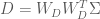
This means that we can transform into an uncorrelated (i.e. orthogonal) set of variables by premultiplying data matrix with the transpose of the the eigenvectors of data covariance matrix .

Whitening: Transforming data to have an Identity Covariance matrix

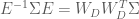
Ok, so now we have a way of transforming our data so that the dimensions are uncorrelated. However, this only gives us a diagonal covariance matrix, not an Identity covariance matrix. In order to obtain an Identity covariance, we also need to scale each dimension so that its variance is equal to one. How can we determine this transformation? We know how to transform our data so that the covariance is equal to . If we can determine the transformation that leaves , then we can apply this transformation to our decorrelated covariance to give us the desired whitening transform. We can determine this from the somewhat trivial notion that

                                                                                                       (8)

and further that

                                                                                            (9)

Now, using Equation (4) along with Equation (8), we can see that

                                                                                     (10)

Now say that we define a variable , where is the desired whitening transform, that leaves the covariance of equal to the identity matrix. Using essentially the same set of derivation steps as above to solve for , but starting from Equation (9) we find that

                                                                                                 (11)

                                                                                                (12)

Thus, the whitening transform is simply the decorrelation transform, but scaled by the inverse of the square root of the (here the inverse and square root can be performed element-wise because is a diagonal matrix).

Interpretation of the Whitening Transform

So what does the whitening transformation actually do to the data (below, blue points)? We investigate this transformation below: The first operation decorrelates the data by premultiplying the data with the eigenvector matrix , calculated from the data covariance. This decorrelation can be thought of as a rotation that reorients the data so that the principal axes of the data are aligned with the axes along which the data has the largest (orthogonal) variance. This rotation is essentially the same procedure as the oft-used Principal Components Analysis (PCA), and is shown in the middle row.

The second operation, scaling by can be thought of squeezing the data–if the variance along a dimension is larger than one–or stretching the data–if the variance along a dimension is less than one. The stretching and squeezing forms the data into a sphere about the origin (which is why whitening is also referred to as “sphering”). This scaling operation is depicted in the bottom row in the plot above.

The MATLAB to make make the plot above is here:

% INITIALIZE SOME CONSTANTS
mu = [0 0];
S = [1 .9; .9 3];

% SAMPLE SOME DATAPOINTS
nSamples = 1000;
samples = mvnrnd(mu,S,nSamples)';

% WHITEN THE DATA POINTS...
[E,D] = eig(S);

% ROTATE THE DATA
samplesRotated = E*samples;

% TAKE D^(-1/2)
D = diag(diag(D).^-.5);

% SCALE DATA BY D
samplesRotatedScaled = D*samplesRotated;

% DISPLAY
figure;

subplot(311);
plot(samples(1,:),samples(2,:),'b.')
axis square, grid
xlim([-5 5]);ylim([-5 5]);
title('Original Data');

subplot(312);
plot(samplesRotated(1,:),samplesRotated(2,:),'r.'),
axis square, grid
xlim([-5 5]);ylim([-5 5]);
title('Decorrelate: Rotate by V');

subplot(313);
plot(samplesRotatedScaled(1,:),samplesRotatedScaled(2,:),'ko')
axis square, grid
xlim([-5 5]);ylim([-5 5]);
title('Whiten: scale by D^{-1/2}');

The transformation in Equation (11) and implemented above  whitens the data but leaves the data aligned with principle axes of the original data. In order to observe the data in the original space, it is often customary “un-rotate” the data back into it’s original space. This is done by just multiplying the whitening transform by the inverse of the rotation operation defined by the eigenvector matrix. This gives the whitening transform:

                                                                                                  (13)

Let’s take a look an example of using statistical whitening for a more complex problem: whitening patches of images sampled from natural scenes.

Example: Whitening Natural Scene Image Patches

Modeling the local spatial structure of pixels in natural scene images is important in many fields including computer vision and computational neuroscience. An interesting model of natural scenes is one that can account for interesting, high-order statistical dependencies between pixels. However, because natural scenes are generally composed of continuous objects or surfaces, a vast majority of the spatial correlations in natural image data can be explained by local pairwise dependencies. For example, observe the image below.

% LOAD AND DISPLAY A NATURAL IMAGE
im = double(imread('cameraman.tif'));
figure
imagesc(im); colormap gray; axis image; axis off;
title('Base Image')

Given one of the gray pixels in the upper portion of the image, it is very likely that all pixels within the local neighborhood will also be gray. Thus there is a large amount of correlation between pixels in local regions of natural scenes. Statistical models of local structure applied to natural scenes will be dominated by these pairwise correlations, unless they are removed by preprocessing. Whitening provides such a preprocessing procedure.

Below we create and display a dataset of local image patches of size extracted at random from the image above. Each patch is rastered out into a column vector of size . Each of these patches can be thought of as samples of the local structure of this natural scene. Below we use the whitening transformation to remove pairwise correlations between pixels in each patch and scale the variance of each pixel to be one.

On the left is the dataset of extracted image patches, along with the corresponding covariance matrix for the image patches on the right. The large local correlation within the neighborhood of each pixel is indicated by the large bright diagonal regions throughout the covariance matrix.

The MATLAB code to extract and display the patches shown above is here:

% CREATE PATCHES DATASET FROM NATURAL IMAGE
rng(12345)
imSize = 256;
nPatches = 400;  % (MAKE SURE SQUARE)
patchSize = 16;
patches = zeros(patchSize*patchSize,nPatches);
patchIm = zeros(sqrt(nPatches)*patchSize);

% PAD IMAGE FOR EDGE EFFECTS
im = padarray(im,[patchSize,patchSize],'symmetric');

% EXTRACT PATCHES...
for iP = 1:nPatches
	pix = ceil(rand(2,1)*imSize);
	rows = pix(1):pix(1)+patchSize-1;
	cols = pix(2):pix(2)+patchSize-1;
	tmp = im(rows,cols);
	patches(:,iP) = reshape(tmp,patchSize*patchSize,1);
	rowIdx = (ceil(iP/sqrt(nPatches)) - 1)*patchSize + ...
                 1:ceil(iP/sqrt(nPatches))*patchSize;
	colIdx = (mod(iP-1,sqrt(nPatches)))*patchSize+1:patchSize* ...
                 ((mod(iP-1,sqrt(nPatches)))+1);
	patchIm(rowIdx,colIdx) = tmp;
end

% CENTER IMAGE PATCHES
patchesCentered = bsxfun(@minus,patches,mean(patches,2));

% CALCULATE COVARIANCE MATRIX
S = patchesCentered*patchesCentered'/nPatches;

% DISPLAY PATCHES
figure;
subplot(121);
imagesc(patchIm);
axis image; axis off; colormap gray;
title('Extracted Patches')

% DISPLAY COVARIANCE
subplot(122);
imagesc(S);
axis image; axis off; colormap gray;
title('Extracted Patches Covariance')

Below we implement the whitening transformation described above to the extracted image patches and display the whitened patches that result.

On the left, we see that the whitening procedure zeros out all areas in the extracted patches that have the same value (zero is indicated by gray). The whitening procedure also boosts the areas of high-contrast (i.e. edges). The right plots the covariance matrix for the whitened patches. The covarance matrix is diagonal, indicating that pixels are now independent. In addition, all diagonal entries have the same value, indicating the that all pixels now have the same variance (i.e. 1). The MATLAB code used to whiten the image patches and create the display above is here:

%% MAIN WHITENING

% DETERMINE EIGENECTORS & EIGENVALUES
% OF COVARIANCE MATRIX
[E,D] = eig(S);

% CALCULATE D^(-1/2)
d = diag(D);
d = real(d.^-.5);
D = diag(d);

% CALCULATE WHITENING TRANSFORM
W = E*D*E';

% WHITEN THE PATCHES
patchesWhitened = W*patchesCentered;

% DISPLAY THE WHITENED PATCHES
wPatchIm = zeros(size(patchIm));
for iP = 1:nPatches
	rowIdx = (ceil(iP/sqrt(nPatches)) - 1)*patchSize + 1:ceil(iP/sqrt(nPatches))*patchSize;
	colIdx = (mod(iP-1,sqrt(nPatches)))*patchSize+1:patchSize* ...
	         ((mod(iP-1,sqrt(nPatches)))+1);
	wPatchIm(rowIdx,colIdx) = reshape(patchesWhitened(:,iP),...
	                                  [patchSize,patchSize]);
end

figure
subplot(121);
imagesc(wPatchIm);
axis image; axis off; colormap gray; caxis([-5 5]);
title('Whitened Patches')

subplot(122);
imagesc(cov(patchesWhitened'));
axis image; axis off; colormap gray; %colorbar
title('Whitened Patches Covariance');

Investigating the Whitening Matrix: implications for theoretical neuroscience

So what does the whitening matrix look like, and what does it do? Below is the whitening matrix calculated for the image patches dataset:

% DISPLAY THE WHITENING MATRIX
figure; imagesc(W);
axis image; colormap gray; colorbar
title('The Whitening Matrix W')

Each column of is the operation that scales the variance of the corresponding pixel to be equal to one and forces that pixel independent of the others in the patch. So what exactly does such an operation look like? We can get an idea by reshaping a column of W back into the shape of the image patches. Below we show what the 86th column of W looks like when reshaped in such a way (the index 86 has no particular significance, it was chosen at random):

% DISPLAY A COLUMN OF THE WHITENING MATRIX
figure; imagesc(reshape(W(:,86),16,16)),
colormap gray,
axis image, colorbar
title('Column 86 of W')

We see that the operation is essentially an impulse centered on the 86th pixel in the image (counting pixels starting in the upper left corner, proceeding down columns). This impulse is surrounded by inhibitory weights. If we were to look at the remaining columns of , we would find that that the same center-surround operation is being replicated at every pixel location in each image patch. Essentially, the whitening transformation is performing a convolution of each image patch with a center-surround filter whose properties are estimated from the patches dataset. Similar techniques are common in computer vision edge-detection algorithms.

Implications for theoretical neuroscience

A theoretical function of the primate retina is data compression: a large number of photoreceptors  pass data from the retina into a physiological bottleneck, the optic nerve, which has far fewer fibers than retinal photoreceptors. Thus removing redundant information is an important task that the retina must perform. When observing the whitened image patches above, we see that redundant information is nullified; pixels that have similar local values to one another are zeroed out. Thus, statistical whitening is a viable form of data compression

It turns out that there is a large class of ganglion cells in the retina whose spatial receptive fields exhibit…that’s right center-surround activation-inhibition like the operation of the whitening matrix shown above! Thus it appears that the primate visual system may be performing data compression at the retina by means of a similar operation to statistical whitening. Above, we derived the center-surround whitening operation based on data sampled from a natural scene. Thus it is seems reasonable that the primate visual system may have evolved a similar data-compression mechanism through experience with natural scenes, either through evolution, or development.

Covariance Matrices and Data Distributions

Correlation between variables in a -dimensional dataset are often summarized by a covariance matrix. To get a better understanding of how correlation matrices characterize correlations between data points, we plot data points drawn from 3 different 2-dimensional Gaussian distributions, each of which is defined by a different covariance matrix.

The left plots below display the covariance matrix for each Gaussian distribution. The values along the diagonal represent the variance of the data along each dimension, and the off-diagonal values represent the covariances between the dimensions. Thus the -th entry of each matrix represents the correlation between the -th and -th dimensions. The right plots show data drawn from the corresponding 2D Gaussian.

The top row plot display a covariance matrix equal to the identity matrix, and the points drawn from the corresponding Gaussian distribution. The diagonal values are 1, indicating the data have variance of 1 along both of the dimensions. Additionally, the off-diagonal elements are zero, meaning that the two dimensions are uncorrelated.  We can see this in the data drawn from the distribution as well. The data are distributed in a sphere about origin. For such a distribution of points, it is difficult (impossible) to draw any single regression line that can predict the second dimension from the first, and vice versa. Thus an identity covariance matrix is equivalent to having independent dimensions, each of which has unit (i.e. 1) variance. Such a dataset is often called “white” (this naming convention comes from the notion that white noise signals–which can be sampled from independent Gaussian distributions–have equal power at all frequencies in the Fourier domain).

The middle row plots the points that result from a diagonal, but not identity covariance matrix. The off-diagonal elements are still zero, indicating that the dimensions are uncorrelated. However, the variances along each dimension are not equal to one, and are not equal. This is demonstrated by the elongated distribution in red. The elongation is along the second dimension, as indicated by the larger value in the bottom-right (point ) of the covariance matrix.

The bottom row plots points that result from a non-diagonal covariance matrix. Here the off-diagonal elements of covariance matrix have non-zero values, indicating a correlation between the dimensions. This correlation is reflected in the distribution of drawn datapoints (in blue). We can see that the primary axis along which the points are distributed is not along either of the dimensions, but a linear combination of the dimensions.

The MATLAB code to create the above plots is here

% INITIALIZE SOME CONSTANTS
mu = [0 0];         % ZERO MEAN
S = [1 .9; .9 3];   % NON-DIAGONAL COV.
SDiag = [1 0; 0 3]; % DIAGONAL COV.
SId = eye(2);       % IDENTITY COV.

% SAMPLE SOME DATAPOINTS
nSamples = 1000;
samples = mvnrnd(mu,S,nSamples)';
samplesId = mvnrnd(mu,SId,nSamples)';
samplesDiag = mvnrnd(mu,SDiag,nSamples)';

% DISPLAY
subplot(321);
imagesc(SId); axis image,
caxis([0 1]), colormap hot, colorbar
title('Identity Covariance')

subplot(322)
plot(samplesId(1,:),samplesId(2,:),'ko'); axis square
xlim([-5 5]), ylim([-5 5])
grid
title('White Data')

subplot(323);
imagesc(SDiag); axis image,
caxis([0 3]), colormap hot, colorbar
title('Diagonal Covariance')

subplot(324)
plot(samplesDiag(1,:),samplesDiag(2,:),'r.'); axis square
xlim([-5 5]), ylim([-5 5])
grid
title('Uncorrelated Data')

subplot(325);
imagesc(S); axis image,
caxis([0 3]), colormap hot, colorbar
title('Non-diagonal Covariance')

subplot(326)
plot(samples(1,:),samples(2,:),'b.'); axis square
xlim([-5 5]), ylim([-5 5])
grid
title('Correlated Data')

fMRI In Neuroscience: Efficiency of Event-related Experiment Designs

Event-related fMRI experiments are used to detect selectivity in the brain to stimuli presented over short durations. An event is generally modeled as an impulse function that occurs at the onset of the stimulus in question. Event-related designs are flexible in that many different classes of stimuli can be intermixed. These designs can minimize confounding behavioral effects due to subject adaptation or expectation. Furthermore, stimulus onsets can be modeled at frequencies that are shorter than the repetition time (TR) of the scanner. However, given such flexibility in design and modeling, how does one determine the schedule for presenting a series of stimuli? Do we space out stimulus onsets periodically across a scan period? Or do we randomize stimulus onsets? Furthermore what is the logic for or against either approach? Which approach is more efficient for gaining incite into the selectivity in the brain?

Simulating Two fMRI Experiments: Periodic and Random Stimulus Onsets

To get a better understanding of the problem of choosing efficient experiment design, let’s simulate two simple fMRI experiments. In the first experiment, a stimulus is presented periodically 20 times, once every 4 seconds, for a run of 80 seconds in duration. We then simulate a noiseless BOLD signal evoked in a voxel with a known HRF. In the second experiment, we simulate the noiseless BOLD signal evoked by 20 stimulus onsets that occur at random times over the course of the 80 second run duration.  The code for simulating the signals and displaying output are shown below:

rand('seed',12345);
randn('seed',12345);
TR = 1 % REPETITION TIME
t = 1:TR:20; % MEASUREMENTS
h = gampdf(t,6) + -.5*gampdf(t,10); % ACTUAL HRF
h = h/max(h); % SCALE TO MAX OF 1

% SOME CONSTANTS...
trPerStim = 4; % # TR PER STIMULUS FOR PERIODIC EXERIMENT
nRepeat = 20; % # OF TOTAL STIMULI SHOWN
nTRs = trPerStim*nRepeat
stimulusTrain0 = zeros(1,nTRs);

beta = 3; % SELECTIVITY/HRF GAIN

% SET UP TWO DIFFERENT STIMULUS PARADIGM...
% A. PERIODIC, NON-RANDOM STIMULUS ONSET TIMES
D_periodic = stimulusTrain0;
D_periodic(1:trPerStim:trPerStim*nRepeat) = 1;

% UNDERLYING MODEL FOR (A)
X_periodic = conv2(D_periodic,h);
X_periodic = X_periodic(1:nTRs);
y_periodic = X_periodic*beta;

% B. RANDOM, UNIFORMLY-DISTRIBUTED STIMULUS ONSET TIMES
D_random = stimulusTrain0;
randIdx = randperm(numel(stimulusTrain0)-5);
D_random(randIdx(1:nRepeat)) = 1;

% UNDERLYING MODEL FOR (B)
X_random = conv2(D_random,h);
X_random = X_random(1:nTRs);
y_random = X_random*beta;

% DISPLAY STIMULUS ONSETS AND EVOKED RESPONSES
% FOR EACH EXPERIMENT
figure
subplot(121)
stem(D_periodic,'k');
hold on;
plot(y_periodic,'r','linewidth',2);
xlabel('Time (TR)');
title(sprintf('Responses Evoked by\nPeriodic Stimulus Onset\nVariance=%1.2f',var(y_periodic)))

subplot(122)
stem(D_random,'k');
hold on;
plot(y_random,'r','linewidth',2);
xlabel('Time (TR)');
title(sprintf('Responses Evoked by\nRandom Stimulus Onset\nVariance=%1.2f',var(y_random)))

BOLD signals evoked by periodic (left) and random (right) stimulus onsets.

The black stick functions in the simulation output indicate the stimulus onsets and each red function is the simulated noiseless BOLD signal to those stimuli. The first thing to notice is the dramatically different variances of the BOLD signals evoked for the two stimulus presentation schedules. For the periodic stimuli, the BOLD signal quickly saturates, then oscillates around an effective baseline activation. The estimated variance of the periodic-based signal is 0.18. In contrast, the signal evoked by the random stimulus presentation schedule varies wildly, reaching a maximum amplitude that is roughly 2.5 times as large the maximum amplitude of the signal evoked by periodic stimuli. The estimated variance of the signal evoked by the random stimuli is 7.4, roughly 40 times the variance of the signal evoked by the periodic stimulus.

So which stimulus schedule allows us to better estimate the HRF and, more importantly, the amplitude of the HRF, as it is the amplitude that is the common proxy for voxel selectivity/activation? Below we repeat the above experiment 50 times. However, instead of simulating noiseless BOLD responses, we introduce 50 distinct, uncorrelated noise conditions, and from the simulated noisy responses, we estimate the HRF using an FIR basis set for each  repeated trial. We then compare the estimated HRFs across the 50 trials for the periodic and random stimulus presentation schedules. Note that for each trial, the noise is exactly the same for the two stimulus presentation schedules. Further, we simulate a selectivity/tuning gain of 3 times the maximum HRF amplitude and assume that the HRF to be estimated is 16 TRs/seconds in length. The simulation and output are below:

%% SIMULATE MULTIPLE TRIALS OF EACH EXPERIMENT
%% AND ESTIMATE THE HRF FOR EACH
%% (ASSUME THE VARIABLES DEFINED ABOVE ARE IN WORKSPACE)

% CREATE AN FIR DESIGN MATRIX
% FOR EACH EXPERIMENT
hrfLen = 16;  % WE ASSUME TO-BE-ESTIMATED HRF IS 16 TRS LONG

% CREATE FIR DESIGN MATRIX FOR THE PERIODIC STIMULI
X_FIR_periodic = zeros(nTRs,hrfLen);
onsets = find(D_periodic);
idxCols = 1:hrfLen;
for jO = 1:numel(onsets)
	idxRows = onsets(jO):onsets(jO)+hrfLen-1;
	for kR = 1:numel(idxRows);
		X_FIR_periodic(idxRows(kR),idxCols(kR)) = 1;
	end
end
X_FIR_periodic = X_FIR_periodic(1:nTRs,:);

% CREATE FIR DESIGN MATRIX FOR THE RANDOM STIMULI
X_FIR_random = zeros(nTRs,hrfLen);
onsets = find(D_random);
idxCols = 1:hrfLen;
for jO = 1:numel(onsets)
	idxRows = onsets(jO):onsets(jO)+hrfLen-1;
	for kR = 1:numel(idxRows);
		X_FIR_random(idxRows(kR),idxCols(kR)) = 1;
	end
end
X_FIR_random = X_FIR_random(1:nTRs,:);

% SIMULATE AND ESTIMATE HRF WEIGHTS VIA OLS
nTrials = 50;

% CREATE NOISE TO ADD TO SIGNALS
% NOTE: SAME NOISE CONDITIONS FOR BOTH EXPERIMENTS
noiseSTD = beta*2;
noise = bsxfun(@times,randn(nTrials,numel(X_periodic)),noiseSTD);

%% ESTIMATE HRF FROM PERIODIC STIMULUS TRIALS
beta_periodic = zeros(nTrials,hrfLen);
for iT = 1:nTrials
	y = y_periodic + noise(iT,:);
	beta_periodic(iT,:) = X_FIR_periodic\y';
end

% CALCULATE MEAN AND STANDARD ERROR OF HRF ESTIMATES
beta_periodic_mean = mean(beta_periodic);
beta_periodic_se = std(beta_periodic)/sqrt(nTrials);

%% ESTIMATE HRF FROM RANDOM STIMULUS TRIALS
beta_random = zeros(nTrials,hrfLen);
for iT = 1:nTrials
	y = y_random + noise(iT,:);
	beta_random(iT,:) = X_FIR_random\y';
end

% CALCULATE MEAN AND STANDARD ERROR OF HRF ESTIMATES
beta_random_mean = mean(beta_random);
beta_random_se = std(beta_random)/sqrt(nTrials);

% DISPLAY HRF ESTIMATES
figure
% ...FOR THE PERIODIC STIMULI
subplot(121);
hold on;
h0 = plot(h*beta,'k')
h1 = plot(beta_periodic_mean,'linewidth',2);
h2 = plot(beta_periodic_mean+beta_periodic_se,'r','linewidth',2);
plot(beta_periodic_mean-beta_periodic_se,'r','linewidth',2);
xlabel('Time (TR)')
legend([h0, h1,h2],'Actual HRF','Average \beta_{periodic}','Standard Error')
title('Periodic HRF Estimate')

% ...FOR THE RANDOMLY-PRESENTED STIMULI
subplot(122);
hold on;
h0 = plot(h*beta,'k');
h1 = plot(beta_random_mean,'linewidth',2);
h2 = plot(beta_random_mean+beta_random_se,'r','linewidth',2);
plot(beta_random_mean-beta_random_se,'r','linewidth',2);
xlabel('Time (TR)')
legend([h0,h1,h2],'Actual HRF','Average \beta_{random}','Standard Error')
title('Random HRF Estimate')

Estimated HRFs from 50 trials of periodic (left) and random (right) stimulus schedules

In the simulation outputs, the average HRF for the random stimulus presentation (right) closely follows the actual HRF tuning. Also, there is little variability of the HRF estimates, as is indicated by the small standard error estimates for each time points. As well, the selectivity/gain term is accurately recovered, giving a mean HRF with nearly the same amplitude as the underlying model. In contrast, the HRF estimated from the periodic-based experiment is much more variable, as indicated by the large standard error estimates. Such variability in the estimates of the HRF reduce our confidence in the estimate for any single trial. Additionally, the scale of the mean HRF estimate is off by nearly 30% of the actual value.

From these results, it is obvious that the random stimulus presentation rate gives rise to more accurate, and less variable estimates of the HRF function. What may not be so obvious is why this is the case, as there were the same number of stimuli and  the same number of signal measurements in each experiment. To get a better understanding of why this is occurring, let’s refer back to the variances of the evoked noiseless signals. These are the signals that are underlying the noisy signals used to estimate the HRF. When noise is added it impedes the detection of the underlying trends that are useful for estimating the HRF.  Thus it is important that the variance of the underlying signal is large compared to the noise so that the signal can be detected.

For the periodic stimulus presentation schedule, we saw that the variation in the BOLD signal was much smaller than the variation in the BOLD signals evoked during the randomly-presented stimuli. Thus the signal evoked by random stimulus schedule provide a better characterization of the underlying signal in the presence of the same amount of noise, and thus provide more information to estimate the HRF. With this in mind we can think of maximizing the efficiency of the an experiment design as maximizing the variance of the BOLD signals evoked by the experiment.

An Alternative Perspective: The Frequency Power Spectrum

Another helpful interpretation is based on a signal processing perspective. If we assume that neural activity is directly correspondent with the onset of a stimulus event, then we can interpret the train of stimulus onsets as a direct signal of the evoked neural activity. Furthermore, we can interpret the HRF as a low-pass-filter that acts to “smooth” the available neural signal in time. Each of these signals–the neural/stimulus signal and the HRF filtering signal–has with it an associated power spectrum. The power spectrum for a signal captures the amount of power per unit time that the signal has as a particular frequency . The power spectrum for a discrete signal can be calculated from the discrete Fourier transform (DFT) of the signal as follows

Below, we use Matlab’s function to calculate the DFT and the associated power spectrum for each of the stimulus/neural signals, as well as the HRF.

%% POWER SPECTRUM ANALYSES
%% (ASSUME THE VARIABLES DEFINED ABOVE ARE IN WORKSPACE)

% MAKE SURE WE PAD SUFFICIENTLY
% FOR CIRCULAR CONVOLUTION
N = 2^nextpow2(nTRs + numel(h)-1);
nUnique = ceil(1+N/2); % TAKE ONLY POSITIVE SPECTRA

% CALCULATE POWER SPECTRUM FOR PERIODIC STIMULI EXPERIMENT
ft_D_periodic = fft(D_periodic,N)/N; % DFT
P_D_periodic = abs(ft_D_periodic).^2; % POWER
P_D_periodic = 2*P_D_periodic(2:nUnique-1); % REMOVE ZEROTH & NYQUIST

% CALCULATE POWER SPECTRUM FOR RANDOM STIMULI EXPERIMENT
ft_D_random = fft(D_random,N)/N; % DFT
P_D_random = abs(ft_D_random).^2; % POWER
P_D_random = 2*P_D_random(2:nUnique-1); % REMOVE ZEROTH & NYQUIST

% CALCULATE POWER SPECTRUM OF HRF
ft_h = fft(h,N)/N; % DFT
P_h = abs(ft_h).^2; % POWER
P_h = 2*P_h(2:nUnique-1); % REMOVE ZEROTH & NYQUIST

% CREATE A FREQUENCY SPACE FOR PLOTTING
F = 1/N*[1:N/2-1];

% DISPLAY STIMULI POWER SPECTRA
figure
subplot(131)
hhd = plot(F,P_D_periodic,'b','linewidth',2);
axis square; hold on;
hhr = plot(F,P_D_random,'g','linewidth',2);
xlim([0 .3]); xlabel('Frequency (Hz)');
set(gca,'Ytick',[]); ylabel('Magnitude');
legend([hhd,hhr],'Periodic','Random')
title('Stimulus Power, P_{stim}')

% DISPLAY HRF POWER SPECTRUM
subplot(132)
plot(F,P_h,'r','linewidth',2);
axis square
xlim([0 .3]); xlabel('Frequency (Hz)');
set(gca,'Ytick',[]); ylabel('Magnitude');
title('HRF Power, P_{HRF}')

% DISPLAY EVOKED SIGNAL POWER SPECTRA
subplot(133)
hhd = plot(F,P_D_periodic.*P_h,'b','linewidth',2);
hold on;
hhr = plot(F,P_D_random.*P_h,'g','linewidth',2);
axis square
xlim([0 .3]); xlabel('Frequency (Hz)');
set(gca,'Ytick',[]); ylabel('Magnitude');
legend([hhd,hhr],'Periodic','Random')
title('Signal Power, P_{stim}.*P_{HRF}')

Power spectrum of neural/stimulus (left), HRF (center), and evoked BOLD (right) signals

On the left of the output we see the power spectra for the stimulus signals. The blue line corresponds to the spectrum for the periodic stimuli, and the green line the spectrum for the randomly-presented stimuli. The large peak in the blue spectrum corresponds to the majority of the stimulus power at 0.25 Hz for the periodic stimuli, as this the fundamental frequency of the periodic stimulus presentation (i.e. every 4 seconds). However, there is little power at any other stimulus frequencies. In contrast the green spectrum indicates that the random stimulus presentation has power at multiple frequencies.

If we interpret the HRF as a filter, then we can think of the HRF power spectrum as modulating the power spectrum of the neural signals to produce the power of the evoked BOLD signals. The power spectrum for the HRF is plotted in red in the center plot. Notice how a majority of the power for the HRF is at frequencies less than 0.1 Hz, and there is very little power at frequencies above 0.2 Hz. If the neural signal power is modulated by the HRF signal power, we see that there is little resultant power in the BOLD signals evoked by periodic stimulus presentation (blue spectrum in the right plot). In contrast, because the power for the neural signals evoked by random stimuli are spread across the frequency domain, there are a number of frequencies that overlap with those frequencies for which the HRF also has power. Thus after modulating neural/stimulus power with the HRF power, the spectrum of the BOLD signals evoked by the randomly-presented stimuli have much more power across the relevant frequency spectrum than those evoked by the periodic stimuli. This is indicated by the larger area under the green curve in the right plot.

Using the signal processing perspective allows us to directly gain perspective on the limitations of a particular experiment design which are rooted in the frequency spectrum of the HRF. Therefore, another way we can think of maximizing the efficiency of an experimental design is maximizing the amount of power in the resulting evoked BOLD responses.

Yet Another Perspective Based in Statistics: Efficiency Metric

Taking a statistics-based approach leads to a formal definition of efficiency, and further, a nice metric for testing the efficiency of an experimental design. Recall that when determining the shape of the HRF, a common approach is to use the GLM model

Here is the evoked BOLD signal and is a design matrix that links a set of linear model parameters to those responses. The variable is a noise term that is unexplained by the model. Using an FIR basis formulation of the model, the weights in represent the HRF to a stimulus condition.

Because fMRI data are a continuous time series, the underlying noise is generally correlated in time. We can model this noise as a Gaussian process with zero mean and a constant multivariate covariance . Note that this is analogous to the Generalized Least Squares (GLS) formulation of the GLM. In general, the values that comprise are unknown and have to be estimated from the fMRI data themselves.

For a known or estimated noise covariance, the Maximum Likelihood Estimator (MLE) for the model parameters (derivation not shown) is:

Because the ML estimator of the HRF is a linear combination of the design matrix and a set of corresponding responses, which are both random variables ( can represent any possible experiment design, and is by definition random), the estimator is itself a random variable. It thus follows that the estimate for the HRF also has a variance. (We demonstrated how is a random variable in the 50 simulations above, where for each simulation X was held fixed, but due to the added noise was a random variable. For each noise condition, the estimate for took on different values.) We saw above how an HRF estimator with a large variance is undesirable, as it reduces our confidence in the estimates of the HRF shape and scale. Therefore we would like to determine an estimator that has a minimum overall variance.

A formal metric for efficiency of a least-squares estimator is directly related to the variance of the estimator. The efficiency is defined to be the inverse of the sum of the estimator variances. An estimator that has a large sum of variances will have a low efficiency, and vice versa. But how do we obtain the values of the variances for the estimator? The variances can be recovered from the diagonal elements of the estimator covariance matrix , giving the following definition for the efficiency,

In earlier post we found that the covariance matrix for the GLS estimator (i.e. the formulation above) with a given noise covariance is:

.

Thus the efficiency for the HRF estimator is

Here we see that the efficiency depends only on the known noise covariance (or an estimate of it), and the design matrix used in the model, but not the shape of the HRF. In general the noise covariance is out of the experimenter’s control (but see the take-homes below ), and must be dealt with post hoc. However, because the design matrix is directly related to the experimental design, the above expression gives a direct way to test the efficiency of experimental designs before they are ever used!

In the simulations above, the noise processes are drawn from an independent multivariate Gaussian distribution, therefore the noise covariance is equal to the identity (i.e. uncorrelated). We also estimated the HRF using the FIR basis set, thus our model design matrix was . This gives the estimate the efficiency for the simulation experiments:

Below we calculate the efficiency for the FIR estimates under the simulated experiments with periodic and random stimulus presentation designs.

%% ESTIMATE DESIGN EFFICIENCY
%% (ASSUME THE VARIABLES DEFINED ABOVE ARE IN WORKSPACE)

% CALCULATE EFFICIENCY OF PERIODIC EXPERIMENT
E_periodic = 1/trace(pinv(X_FIR_periodic'*X_FIR_periodic));

% CALCULATE EFFICIENCY OF RANDOM EXPERIMENT
E_random = 1/trace(pinv(X_FIR_random'*X_FIR_random));

% DISPLAY EFFICIENCY ESTIMATES
figure
bar([E_periodic,E_random]);
set(gca,'XTick',[1,2],'XTickLabel',{'E_periodic','E_random'});
title('Efficiency of Experimental Designs');
colormap hot;

Estimated efficiency for simulated periodic (left) and random (right) stimulus schedules.

Here we see that the efficiency metric does indeed indicate that the randomly-presented stimulus paradigm is far more efficient than the periodically-presented paradigm.

Wrapping Up

In this post we addressed the efficiency of an fMRI experiment design. A few take-homes from the discussion are:

1. Randomize stimulus onset times. These onset times should take into account the low-pass characteristics (i.e. the power spectrum) of the HRF.
2. Try to model selectivity to events that occur close in time. The reason for this is that noise covariances in fMRI are highly non-stationary. There are many sources of low-frequency physiological noise such as breathing, pulse, blood pressure, etc, all of which dramatically effect the noise in the fMRI timecourses. Thus any estimate of noise covariances from data recorded far apart in time will likely be erroneous.
3. Check an experimental design against other candidate designs using the Efficiency metric.

Above there is mention of the effects of low-frequency physiological noise. Until now, our simulations have assumed that all noise is independent in time, greatly simplifying the picture of estimating HRFs and corresponding selectivity. However, in a later post we’ll address how to deal with more realistic time courses that are heavily influenced by sources of physiological noise. Additionally, we’ll tackle how to go about estimating the noise covariance from more realistic fMRI time series.

Derivation: The Covariance Matrix of an OLS Estimator (and applications to GLS)

We showed in an earlier post that for the linear regression model

,

the optimal Ordinary Least Squares (OLS) estimator for model parameters is

However, because independent variables and responses can take on any value, they are both random variables. And, because is a linear combination of and , it is also a random variable, and therefore has a covariance. The definition of the covariance matrix for the OLS estimator is defined as:

where, denotes the expected value operator. In order to find an expression for , we first need an expression for  . The following derives this expression:

,

where we use the fact that

.

It follows that

and therefore

Now following the original definition for …

where we take advantage of in order to rewrite the second term in the product of the expectation. If we take to be fixed for a given estimator of (in other words we don’t randomly resample the independent variables), then the expectation only depends on the remaining stochastic/random variable, namely . Therefore the above expression can be written as

.

where is the covariance of the noise term in the model. Because OLS assumes uncorrelated noise, the noise covariance is equal to , where is the variance along each dimension, and is an identity matrix of size equal to the number of dimensions. The expression for the estimator covariance is now:

,

which simplifies to

A further simplifying assumption made by OLS that is often made is that is drawn from a zero mean multivariate Guassian distribution of unit variances (i.e. ), resulting in a noise covariance equal to the identity. Thus

Applying the derivation results to Generalized Least Squares

Notice that the expression for the OLS estimator covariance is equal to first inverse term in the expression for the OLS estimator. Identitying the covariance for the OLS estimator in this way gives a helpful heuristic to easily identify the covariance of related estimators that do not make the simplifying assumptions about the covariance that are made in OLS. For instance in Generalized Least Squares (GLS), it is possible for the noise terms to co-vary. The covariance is represented as a noise covariance matrix . This gives the model form

,

where .

In otherwords, under GLS, the noise terms have zero mean, and covariance .  It turns out that estimator for the GLS model parameters is

.

Notice the similarity between the GLS and OLS estimators. The only difference is that in GLS, the solution for the parameters is scaled by the inverse of the noise covariance. And, in a similar fashion to the OLS estimator, the covariance for the GLS estimator is first term in the product that defines the GLS estimator: