MCMC: Hamiltonian Monte Carlo (a.k.a. Hybrid Monte Carlo)

The random-walk behavior of many Markov Chain Monte Carlo (MCMC) algorithms makes Markov chain convergence to a target stationary distribution inefficient, resulting in slow mixing. Hamiltonian/Hybrid Monte Carlo (HMC), is a MCMC method that adopts physical system dynamics rather than a probability distribution to propose future states in the Markov chain. This allows the Markov chain to explore the target distribution much more efficiently, resulting in faster convergence. Here we introduce basic analytic and numerical concepts for simulation of Hamiltonian dynamics. We then show how Hamiltonian dynamics can be used as the Markov chain proposal function for an MCMC sampling algorithm (HMC).

First off, a brief physics lesson in Hamiltonian dynamics

Before we can develop Hamiltonian Monte Carlo, we need to become familiar with the concept of Hamiltonian dynamics. Hamiltonian dynamics is one way that physicists describe how objects move throughout a system. Hamiltonian dynamics describe an object’s motion in terms of its location and momentum (equivalent to the object’s mass times its velocity) at some time . For each location the object takes, there is an associated potential energy , and for each momentum there is an associated kinetic energy . The total energy of the system is constant and known as the Hamiltonian , defined simply as the sum of the potential and kinetic energies:

Hamiltonian dynamics describe how kinetic energy is converted to potential energy (and vice versa) as an object moves throughout a system in time. This description is implemented quantitatively via a set of differential equations known as the Hamiltonian equations:

Therefore, if we have expressions for and and a set of initial conditions (i.e. an initial position and initial momentum at time ), it is possible to predict the location and momentum of an object at any point in time by simulating these dynamics for a duration

Simulating Hamiltonian dynamics — the Leap Frog Method

The Hamiltonian equations describe an object’s motion in time, which is a continuous variable. In order to simulate Hamiltonian dynamics numerically on a computer, it is necessary to approximate the Hamiltonian equations by discretizing  time. This is done by splitting the interval up into a series of smaller intervals of length . The smaller the value of the closer the approximation is to the dynamics in continuous time. There are a number of procedures that have been developed for discretizing time including Euler’s method and the Leap Frog Method, which I will introduce briefly in the context of Hamiltonian dynamics. The Leap Frog method updates the momentum and position variables sequentially, starting by simulating the momentum dynamics over a small interval of time , then simulating the position dynamics over a slightly longer interval in time , then completing the momentum simulation over another small interval of time so that and now exist at the same point in time. Specifically, the Leap Frog method is as follows: 1. Take a half step in time to update the momentum variable:

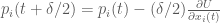
2. Take a full step in time to update the position variable

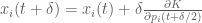
3. Take the remaining half step in time to finish updating the momentum variable

The Leap Fog method can be run for steps to simulate dynamics over units of time. This particular discretization method has a number of properties that make it preferable to other approximation methods like Euler’s method, particularly for use in MCMC, but discussion of these properties are beyond the scope of this post. Let’s see how we can use the Leap Frog method to simulate Hamiltonian dynamics in a simple 1D example.

Example 1: Simulating Hamiltonian dynamics of an harmonic oscillator

Imagine a ball with mass equal to one is attached to a horizontally-oriented spring. The spring exerts a force on the ball equal to

which works to restore the ball’s position to the equilibrium position of the spring  at . Let’s assume that the spring constant , which defines the strength of the restoring force is also equal to one. If the ball is displaced by some distance from equilibrium, then the potential energy is

In addition, the kinetic energy an object with mass moving with velocity within a linear system is known to be

,

if the object’s mass is equal to one, like the ball this example. Notice that we now have in hand the expressions for both and . In order to simulate the Hamiltonian dynamics of the system using the Leap Frog method, we also need expressions for the partial derivatives of each variable (in this 1D example there are only one for each variable):

Therefore one iteration the Leap Frog algorithm for simulating Hamiltonian dynamics in this system is:

1.  
2. 3.

We simulate the dynamics of the spring-mass system described using the Leap Frog method in Matlab below (if the graph is not animated, try clicking on it to open up the linked .gif). The left bar in the bottom left subpanel of the simulation output demonstrates the trade-off between potential and kinetic energy described by Hamiltonian dynamics. The cyan portion of the bar is the proportion of the Hamiltonian contributed by  the potential energy , and the yellow portion  represents is the contribution of the kinetic energy . The right bar (in all yellow), is the total value of the Hamiltonian . Here we see that the ball oscillates about the equilibrium position of the spring with a constant period/frequency.  As the ball passes the equilibrium position , it has a minimum potential energy and maximum kinetic energy. At the extremes of the ball’s trajectory, the potential energy is at a maximum, while the kinetic energy is minimized. The  procession of momentum and position map out positions in what is referred to as phase space, which is displayed in the bottom right subpanel of the output. The harmonic oscillator maps out an ellipse in phase space. The size of the ellipse depends on the energy of the system defined by initial conditions.

Simple example of Hamiltonian Dynamics: 1D Harmonic Oscillator (Click to see animated)

You may also notice that the value of the Hamiltonian is not a exactly constant in the simulation, but oscillates slightly. This is an artifact known as energy drift due to approximations used to the discretize time.

% EXAMPLE 1: SIMULATING HAMILTONIAN DYNAMICS
%            OF HARMONIC OSCILLATOR
% STEP SIZE
delta = 0.1;

% # LEAP FROG
L = 70;

% DEFINE KINETIC ENERGY FUNCTION
K = inline('p^2/2','p');

% DEFINE POTENTIAL ENERGY FUNCTION FOR SPRING (K =1)
U = inline('1/2*x^2','x');

% DEFINE GRADIENT OF POTENTIAL ENERGY
dU = inline('x','x');

% INITIAL CONDITIONS
x0 = -4; % POSTIION
p0 = 1;  % MOMENTUM
figure

%% SIMULATE HAMILTONIAN DYNAMICS WITH LEAPFROG METHOD
% FIRST HALF STEP FOR MOMENTUM
pStep = p0 - delta/2*dU(x0)';

% FIRST FULL STEP FOR POSITION/SAMPLE
xStep = x0 + delta*pStep;

% FULL STEPS
for jL = 1:L-1
	% UPDATE MOMENTUM
	pStep = pStep - delta*dU(xStep);

	% UPDATE POSITION
	xStep = xStep + delta*pStep;

	% UPDATE DISPLAYS
	subplot(211), cla
	hold on;
	xx = linspace(-6,xStep,1000);
	plot(xx,sin(6*linspace(0,2*pi,1000)),'k-');
	plot(xStep+.5,0,'bo','Linewidth',20)
	xlim([-6 6]);ylim([-1 1])
	hold off;
	title('Harmonic Oscillator')
	subplot(223), cla
	b = bar([U(xStep),K(pStep);0,U(xStep)+K(pStep)],'stacked');
	set(gca,'xTickLabel',{'U+K','H'})
	ylim([0 10]);
	title('Energy')
	subplot(224);
	plot(xStep,pStep,'ko','Linewidth',20);
        xlim([-6 6]); ylim([-6 6]); axis square
	xlabel('x'); ylabel('p');
	title('Phase Space')
	pause(.1)
end
% (LAST HALF STEP FOR MOMENTUM)
pStep = pStep - delta/2*dU(xStep);

Hamiltonian dynamics and the target distribution

Now that we have a better understanding of what Hamiltonian dynamics are and how they can be simulated, let’s now discuss how we can use Hamiltonian dynamics for MCMC. The main idea behind Hamiltonian/Hibrid Monte Carlo is to develop a Hamiltonian function such that the resulting Hamiltonian dynamics allow us to efficiently explore some target distribution . How can we choose such a Hamiltonian function? It turns out it is pretty simple to relate a to using a basic concept adopted from statistical mechanics known as the canonical distribution. For any energy function over a set of variables , we can define the corresponding canonical distribution as: where we simply take the exponential of the negative of the energy function. The variable is a normalizing constant called the partition function that scales the canonical distribution such that is sums to one, creating a valid probability distribution. Don’t worry about , it isn’t really important because, as you may recall from an earlier post, MCMC methods can sample from unscaled probability distributions. Now, as we saw above, the energy function for Hamiltonian dynamics is a combination of potential and kinetic energies:

Therefore the canoncial distribution for the Hamiltonian dynamics energy function is

Here we see that joint (canonical) distribution for and factorizes. This means that the two variables are independent, and the canoncial distribution is independent of the analogous distribution for the momentum. Therefore, as we’ll see shortly, we can use Hamiltonian dynamics to sample from the joint canonical distribution over and and simply ignore the momentum contributions. Note that this is an example of introducing auxiliary variables to facilitate the Markov chain path. Introducing the auxiliary variable allows us to use Hamiltonian dynamics, which are unavailable without them. Because the canonical distribution for is independent of the canonical distribution for , we can choose any distribution from which to sample the momentum variables. A common choice is to use a zero-mean Normal distribution with unit variance:

Note that this is equivalent to having a quadratic potential energy term in the Hamiltonian:

Recall that this is is the exact quadratic kinetic energy function (albeit in 1D) used in the harmonic oscillator example above. This is a convenient choice for the kinetic energy function as all partial derivatives are easy to compute. Now that we have defined a kinetic energy function, all we have to do is find a potential energy function that when negated and run through the exponential function, gives the target distribution (or an unscaled version of it). Another way of thinking of it is that we can define the potential energy function as

.

If we can calculate , then we’re in business and we can simulate Hamiltonian dynamics that can be used in an MCMC technique.

Hamiltonian Monte Carlo

In HMC we use Hamiltonian dynamics as a proposal function for a Markov Chain in order to explore the target (canonical) density  defined by more efficiently than using a proposal probability distribution. Starting at an initial state , we simulate Hamiltonian dynamics for a short time using the Leap Frog method. We then use the state of the position and momentum variables at the end of the simulation as our proposed states variables and . The proposed state is accepted using an update rule analogous to the Metropolis acceptance criterion. Specifically if the probability of the proposed state after Hamiltonian dynamics

is greater than probability of the state prior to the Hamiltonian dynamics

then the proposed state is accepted, otherwise, the proposed state is accepted randomly. If the state is rejected, the next state of the Markov chain is set as the state at . For a given set of initial conditions, Hamiltonian dynamics will follow contours of constant energy in phase space (analogous to the circle traced out in phase space in the example above). Therefore we must randomly perturb the dynamics so as to explore all of . This is done by simply drawing a random momentum from the corresponding canonical distribution  before running the dynamics prior to each sampling iteration . Combining these steps, sampling random momentum, followed by Hamiltonian dynamics and Metropolis acceptance criterion defines the HMC algorithm for drawing samples from a target distribution:

1. set
2. generate an initial position state
3. repeat until

set

– sample a new initial momentum variable from the momentum canonical distribution

– set

– run Leap Frog algorithm starting at  for steps and stepsize to obtain proposed states and

– calculate the Metropolis acceptance probability:

– draw a random number from

if accept the proposed state position and set the next state in the Markov chain

else set

In the next example we implement HMC  to sample from a multivariate target distribution that we have sampled from previously using multi-variate Metropolis-Hastings, the bivariate Normal. We also qualitatively compare the sampling dynamics of HMC to multivariate Metropolis-Hastings for the sampling the same distribution.

Example 2: Hamiltonian Monte for sampling a Bivariate Normal distribution

As a reminder, the target distribution for this exampleis a Normal form with following parameterization:

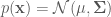
with mean

and covariance

In order to sample from (assuming that we are using a quadratic energy function), we need to determine the expressions for and

.

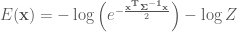
Recall that the target potential energy function can be defined from the canonical form as

If we take the negative log of the Normal distribution outline above, this defines the following potential energy function:

Where is the normalizing constant for a Normal distribution (and can be ignored because it will eventually cancel). The potential energy function is then simply:

with partial derivatives

Using these expressions for the potential energy and its partial derivatives, we implement HMC for sampling from the bivariate Normal in Matlab:

Hybrid Monte Carlo Samples from bivariate Normal target distribution

In the graph above we display HMC samples of the target distribution, starting from an initial position very far from the mean of the target. We can see that HMC rapidly approaches areas of high density under the target distribution. We compare these samples with samples drawn using the Metropolis-Hastings (MH) algorithm below. The MH algorithm converges much slower than HMC, and consecutive samples have much higher autocorrelation than samples drawn using HMC.

Metropolis-Hasting (MH) samples of the same target distribution. Autocorrelation is evident. HMC is much more efficient than MH.

The Matlab code for the HMC sampler:

% EXAMPLE 2: HYBRID MONTE CARLO SAMPLING -- BIVARIATE NORMAL
rand('seed',12345);
randn('seed',12345);

% STEP SIZE
delta = 0.3;
nSamples = 1000;
L = 20;

% DEFINE POTENTIAL ENERGY FUNCTION
U = inline('transp(x)*inv([1,.8;.8,1])*x','x');

% DEFINE GRADIENT OF POTENTIAL ENERGY
dU = inline('transp(x)*inv([1,.8;.8,1])','x');

% DEFINE KINETIC ENERGY FUNCTION
K = inline('sum((transp(p)*p))/2','p');

% INITIAL STATE
x = zeros(2,nSamples);
x0 = [0;6];
x(:,1) = x0;

t = 1;
while t < nSamples
	t = t + 1;

	% SAMPLE RANDOM MOMENTUM
	p0 = randn(2,1);

	%% SIMULATE HAMILTONIAN DYNAMICS
	% FIRST 1/2 STEP OF MOMENTUM
	pStar = p0 - delta/2*dU(x(:,t-1))';

	% FIRST FULL STEP FOR POSITION/SAMPLE
	xStar = x(:,t-1) + delta*pStar;

	% FULL STEPS
	for jL = 1:L-1
		% MOMENTUM
		pStar = pStar - delta*dU(xStar)';
		% POSITION/SAMPLE
		xStar = xStar + delta*pStar;
	end

	% LAST HALP STEP
	pStar = pStar - delta/2*dU(xStar)';

	% COULD NEGATE MOMENTUM HERE TO LEAVE
	% THE PROPOSAL DISTRIBUTION SYMMETRIC.
	% HOWEVER WE THROW THIS AWAY FOR NEXT
	% SAMPLE, SO IT DOESN'T MATTER

	% EVALUATE ENERGIES AT
	% START AND END OF TRAJECTORY
	U0 = U(x(:,t-1));
	UStar = U(xStar);

	K0 = K(p0);
	KStar = K(pStar);

	% ACCEPTANCE/REJECTION CRITERION
	alpha = min(1,exp((U0 + K0) - (UStar + KStar)));

	u = rand;
	if u < alpha
		x(:,t) = xStar;
	else
		x(:,t) = x(:,t-1);
	end
end

% DISPLAY
figure
scatter(x(1,:),x(2,:),'k.'); hold on;
plot(x(1,1:50),x(2,1:50),'ro-','Linewidth',2);
xlim([-6 6]); ylim([-6 6]);
legend({'Samples','1st 50 States'},'Location','Northwest')
title('Hamiltonian Monte Carlo')

Wrapping up

In this post we introduced the Hamiltonian/Hybrid Monte Carlo algorithm for more efficient MCMC sampling. The HMC algorithm is extremely powerful for sampling distributions that can be represented terms of a potential energy function and its partial derivatives. Despite the efficiency and elegance of HMC, it is an underrepresented sampling routine in the literature. This may be due to the popularity of simpler algorithms such as Gibbs sampling or Metropolis-Hastings, or perhaps due to the fact that one must select hyperparameters such as the number of Leap Frog steps and Leap Frog step size when using HMC. However, recent research has provided effective heuristics such as adapting the Leap Frog step size in order to maintain a constant Metropolis rejection rate, which facilitate the use of HMC for general applications.